CT Segmentation

Based on XMapTools 4.5 embedded documentation – Help file version 11.01.2024

---

This page describes the tools available in the Segment section. These tools are optimised for CT data and should not be used with other data types.

The processing of CT data for segmentation is divided into five steps:

1. Create a segmentation scheme
2. Setting the segmentation parameters
3. Testing the segmentation
4. Applying the segmentation and creating a ROI
5. Exporting the results

Step 1 – Segmentation Scheme

A segmentation scheme is a set of recipes containing constraints that are applied to perform data segmentation. It is similar to the training sets for classification, although it does not (yet) contain training data.

Segmentation schemes are available in the secondary menu under Segmentation & Corrections in Schemes (Segmentation).

Select a CT image under the CT Data node in the primary menu and select the Schemes (Segmentation) item in the secondary menu.

The Add (Scheme / Group / Range) button has various functions depending on the item selected in the secondary menu:

• Add a Segmentation Schema when the Schemes (Segmentation) node is selected
• Add a Group Definition when a Segmentation Scheme is selected
• Select a range of values from the displayed values when a group definition is selected. Adjust the min-max values to select a mineral or group of minerals and press Add. A single range of values can be selected for each group, so any new selection would replace existing data

INFO

Selected regions may overlap, but the algorithm will always consider the group in a sequential order. Pixels may be ignored by the segmentation algorithm if they are out of range.

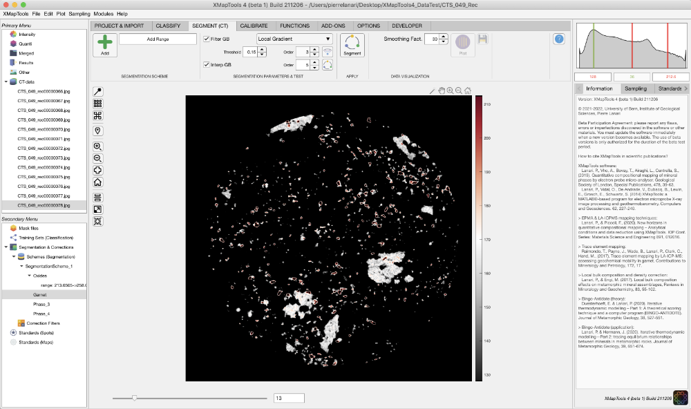
Figure 1: Example of selecting a range of values (here from 128 to 212.6) for garnet. Note that this range has been stored in the segmentation scheme shown in the secondary menu.

Step 2 – Segmentation Parameters

These parameters can be set in the Segment (CT) and Segmentation Parameters & Test sections. There are two main algorithms implemented: Filter GB to remove grain boundaries and Interp GB to remove growth phases and re-interpolate filtered pixels.

Filter Grain Boundaries

Select a CT image from the CT Data node in the primary menu and a segmentation scheme from the secondary menu.

Four algorithms are available and can be selected from a drop-down menu:

• Local Gradient
• Local Standard Deviation
• Local Range
• Local Entropy

You can set the threshold (range between 0 and 1) above which a grain boundary is detected and the order (for the local range).

The Calculate GB map button opens a new figure containing two plots (e.g. Fig. 2): the result of the algorithm on the left and the same map with the filtered grain boundaries shown in red on the right. The axes of the two plots are aligned, and zooming in on one plot automatically adjusts the view of the second plot.

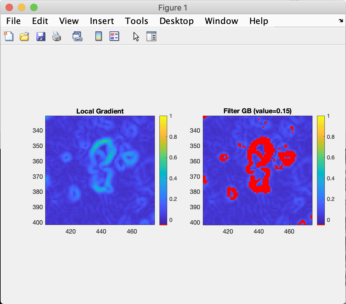
Figure 2: Example of a grain boundary filter using the Local Gradient algorithm and a filter threshold of 0.15. Zoom has been used to show a small part of the image.

Interpolate Grain Boundaries

An algorithm based on a median filter is used to re-interpolate the grain boundary (an equivalent was available in XMapTools 3). The order of interpolation is adjustable.

Step 3 – Segmentation Test

You can test the segmentation on the selected image using the Segment Selected Image (small) button available in Segmentation Parameters & Test.

The resulting ROI is available in the ROI category of the primary menu.

Step 4 – Final Segmentation

The Segment All Images button applies the segmentation to all images available in CT-data. The resulting ROI is available in the ROI category of the primary menu.

Step 5 – Exporting Results

Select a multi-slice ROI (3D ROI) from the primary menu.

The Plot Phase Proportions button generates several plots to examine the spatial distribution of the segmented groups:

1. Evolution of modes from top (left) to bottom (right)
2. Correlation matrix between modes across vertical slices
3. Smooth modal changes (vertical) calculated using the smoothing factor (number of slices to average to calculate a single position)
4. Correlation matrix between smoothed modes over vertical slices