XMapTools documentation for LA-ICP-MS
Table of contents
File format
The importer module should be able to read files in the following format. Note that some format require a conversion before to be imported in XMapTools.
Agilent
The date and time are read from the third row.
D:\Agilent\ICPMH\1\DATA\Name\map.b\map.d
Intensity Vs Time,CPS
Acquired      : 2022-01-24 11:11:45 AM using Batch map.b
Time [Sec],Li7,Na23,Mg25
0.6196,50.00,82227.81,0.00
1.1516,50.00,79613.57,0.00
[...]
Thermo Fisher CSV
The Date and time are read from the first row.
Standards run :02-27-2024 11:16:40 AM;
Software: [...]
Configuration: [...]
S-SQ-N%2FA: [...]
RF Generator: [...]
Ion Optics: [...]
Vacuum: [...]
Detector: [...]
Cooling System: [...]
Power Supply: [...]
Gas Supply: [...]
Pulse Counting: [...]

Time,7Li,23Na,24Mg,25Mg,
,dwell time=0.01;xcal factor=59347.84333,dwell time=0.001;xcal factor=72480.60121,dwell time=0.01;xcal factor=73115.42471
0.01326,400.006400102402,89317.9719802497,0
0.41544,0,67180.0425139374,0
0.81759,0,76231.74450329,0
[...]
Thermo Fisher FIN2
Warning: This file must be converted to CSV format using the 'Tools > Convert FIN2 to CSV' option in the converter.
The Date and time are read from the first row.
Finnigan MAT ELEMENT Raw Data
Friday, July 04, 2025 11:31:12
2025_07_04_Name1.FIN
231
0
16,16,16
CPS
Time,Li7,B10,B11
3.236000,340192.875000,585.555542,887.700012
4.044000,342415.125000,459.555542,934.299988
[...]
Perkin Elmer
The date and time are read from the file timestamp.
Intensity Vs Time, Counts per Second
Time in Seconds ,Mg/25,Al/27,P/31,Ca/42

0.,200.0016000128,1000.0400016001,3067.0428905946,31639.99295109
0.28,200.0016000128,1600.102406554,3267.0935668927,30837.992406645
[...]
Converter for LA-ICP-MS data
The Converter for LA-ICP-MS data can read LA-ICP-MS mapping data natively and generate intensity and standard maps for XMapTools (Markmann et al. 2024).
Main steps to import LA-ICP-MS data:
- Import files including a data file from the mass spectrometer containing timestamps and intensity data, and optionally a log file from the laser system
- Adjust the time shift to synchronise the two data sets
- Generate a log file (if not available) using the Log Generator module
- Extract integrations for each measurement
- Apply a background correction using one of the available functions
- Select primary standard(s) and fit to generate a primary standard intensity function
- Select secondary standard(s) and check the quality of standardisation for each element selected as an internal standard
- Generate maps using the interpolation method described in Markmann et al. (2024) for unknowns and standards, and export map files.
Step 1: Load datafile(s)
The import tools are located at the top of the module. The data format can be selected from the first dropdown menu and the file format (single or multiple) from the second dropdown menu. The data from a measurement session can be contained in a single file or multiple files. If multiple files are selected, it is recommended that you select the last file first and then hold SHIFT while selecting the first file, not vice versa. For the laser, deselect the log file option if no compatible log file is available. In this case, the Log Generator module will appear when the Load Datafiles button is pressed.
Once appropriate options have been selected, press the Load Datafiles button to select: (1) a single data file from the mass spectrometer containing timestamps and intensity data (e.g. Data.csv) or multiple files (see warning above), and (2) if the Log File option is enabled, immediately after a corresponding log file (e.g. Log.csv) from the laser system (tested with RESONETICS only).
Step 2: Adjust time shift
The value of the time shift can be adjusted to synchronise the data file with the log file. In the main figure, the total signal is plotted together with the laser on/off signals given in the log file (vertical red lines). The shift value is automatically adjusted by XMapTools when the data is imported. If necessary, adjust the value until both signals are synchronised.
Step 3: Extract integrations & plot data
Once the value of the time shift is optimised, press the Extract Integrations button to automatically extract all the analyses listed in the log file. They should appear in the Integration tree menu on the left of the window after extraction.
Step 4: Apply background correction
The integrations for fitting a background correction are automatically selected for each measurement. They are listed in a tree menu (integration menu) located on the left and can be plotted by selecting an item under the category Background.
Display/edit integrations for background
To view and edit integrations, select the first measurement in the tree menu. The display is automatically adjusted to zoom in on the selected integration. If you select a different measurement in the tree menu, the integration will be displayed in the centre of the plot. The program automatically excludes a fraction of sweeps at the beginning and at the end of each background measurement (default value is 10 %). This value can be changed manually if required. It is also possible to manually edit the duration of an integration by changing the limit values available as Sweep (min and max).
Background interpolation
Select a method for fitting the background in the BACKGROUND section below the plot. It is recommended to display the signal Raw_Sum and to adjust the display to show the entire background signal. The following functions are available: (1) linear, (2) polynomial, (3) step function, (4) spline. Step function is recommended for background correction. Press the button Apply to apply the background correction. You cannot change the background correction once it has been applied.
Step 5: Select primary standard(s)
The background-corrected (BackCorr) signal is displayed when a background correction has been applied. Corrected data are available from the Plot menu. Select the measurement to be used as the primary standard from the PRIMARY STANDARD dropdown menu. The integration name should match the name of a standard file containing the composition of this standard (e.g. NIST612 or GSD-1g). It is also possible to add custom files using the options available in the lower left panel, but this process must be repeated each time the converter is used. Integrations can be edited using the same strategy as for background integration (see above).
Then select an interpolation method. A spline function is usually the best method to approximate instrument drift during the measurement, especially when reconstructing maps (Markmann et al. 2024). A step function can also be used in some cases, but this can result in sharp transitions between lines in the final map. Press the Apply button to validate and interpolate the primary standard signal. If the standard is not automatically recognised, a window will open with a list of all available standards. It is possible to define additional interpolations to be used as primary standards. After pressing the Apply button it is possible to define a new interpolation for the same material or for a different material by selecting the Yes option. If you do not wish to define any further interpolations to be used as primary standards, select No (Continue).
Step 6: Select and check secondary standard
Select the measurements to be used as the secondary standard using the dropdown menu under SECONDARY STANDARD. Integrations can be edited using the same strategy as for background integration and primary standard (see above). Use the Int. Std dropdown menu to select an element to be used as a reference for calculating the composition of the secondary standard. This choice has no effect at this stage on the map calibration performed in XMapTools (another element can be used). But here it is possible to quickly check the calibration using the secondary standard for several elements used as internal standard.
Step 7: Generate map files
Maps can be generated from raster measurements after background correction, adjustment of the primary reference material(s) and checking of the secondary reference material(s). Use the dropdown menu in MAPS (SCANS) to select the raster measurements to be used to construct the map. Integrations cannot be edited. Press the Apply button to validate and generate the maps. Three buttons become available.
References
Markmann, T.A., Lanari, P., Piccoli, F., Pettke, T., Tamblyn, R., Tedeschi, M., Lueder, M., Kunz, B., Riel, N., and Laughton, J. (2024). Multi-phase quantitative compositional mapping by LA-ICP-MS: analytical approach and data reduction protocol implemented in XMapTools. Chemical Geology, 646, 121895.
For more detailed information on the LA-ICPMS Converter, refer to the embedded documentation available within the program.
Log generator module
When the log generator module is used the time shift should be set to zero.
Calibration
Intensity maps obtained by LA-ICPMS can be calibrated to element/oxide compositions. The following steps can be followed:
- Import standard maps
- Calibrate intensity data
- Generate spider plots
Import standard maps
Only standard maps generated by the Converter for LA-ICPMS data can be imported and used to calibrate LA-ICPMS maps in XMapTools 4.
The button Import (Import Maps for Standards (from file)) is used to open a window in which the file 'MapStandards_Import.mat' must be selected.
Once standard data are imported they become available under the category Standards (Maps) in the Secondary Menu. Select an element to plot a map corresponding to the intensity of the primary standard material.
Calibrate intensity data
As for EPMA, the calibration tool for LA-ICPMS data requires a mask file, so the Calibrate button is only available when a mask file is selected in the Secondary Menu.
The button Calibrate (Open LA-ICP-MS Calibration Tools) opens the calibration assistant.
For more detailed information on the Calibration Assistant, refer to the embedded documentation accessible from the assistant.
Calibration assistant (LA-ICPMS)
The approach implemented in XMapTools 4, described in Markmann et al. (2024), provides a mineral calibration module based on the reference composition of an element (internal standard). In contrast to other programs, the composition of the reference element in the mineral can be variable.
Markmann, T.A., Lanari, P., Piccoli, F., Pettke, T., Tamblyn, R., Tedeschi, M., Lueder, M., Kunz, B., Riel, N., and Laughton, J. (2024). Multi-phase quantitative compositional mapping by LA-ICP-MS: analytical approach and data reduction protocol implemented in XMapTools. Chemical Geology, 646, 121895.
Step-by-step guide
- Select the mineral to be calibrated using the drop-down menu Mineral
- Select the element to be used as the internal standard from the drop-down menu Internal Standard
- Decide whether you want to use a fixed or variable composition using one of the options Fixed composition or Variable composition (see below)
Case 1: Fixed composition
This mode is useful when an element is chemically unzoned in the selected mineral and you want to use it as an internal standard (e.g. SiO₂ in garnet).
You can use the Internal Composition Converter tool to convert the composition of the internal standard into µg/g of element. Enter a value in oxide wt% and the converter will automatically convert this value to µg/g. Note that the value in the Fixed Composition field changes when a new conversion is performed; there is no need to copy the value from one field to the other.
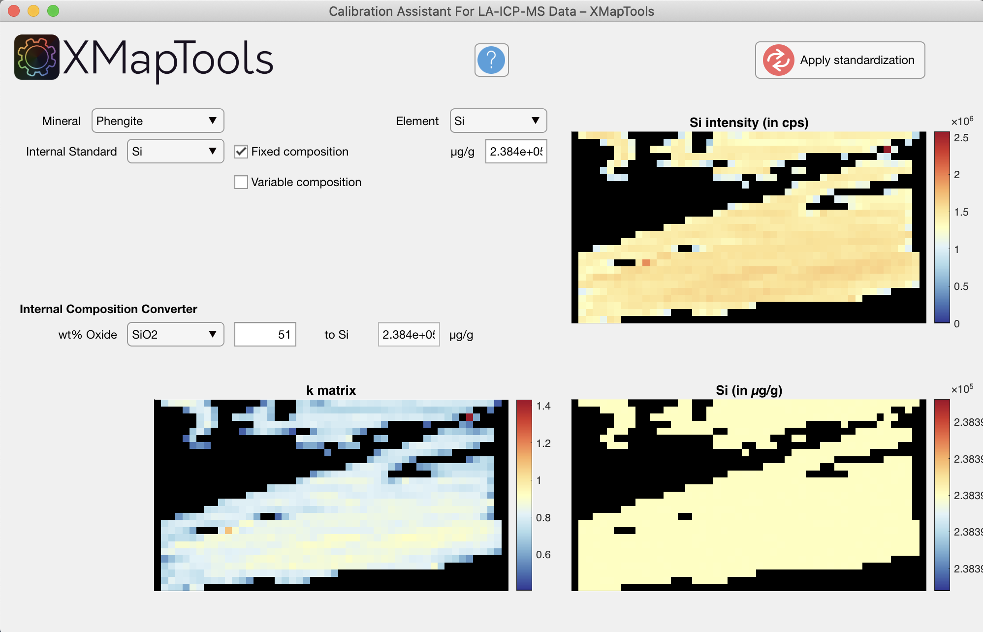
Figure 1: Calibration Assistant for LA-ICPMS data. Example of internal calibration of phengite using Si as internal standard and a reference composition of SiO2 = 51 wt%. The value of Si = 2.384e+05 µg/g has been automatically set in the "Fixed Composition" field. Two maps are displayed at the bottom: the k-matrix calculated using the internal standard and the calibrated map for Si expressed in µg/g.
Press the Apply Standardisation button to generate the compositional maps available in the Quantity category of the Primary Menu. The maps are expressed in µg/g of elements. You can convert them to wt% of oxides using the internal converter: right-click on a Quanti file and select Convert.
TIP
After converting the maps, the name of the maps can be changed (this is not done by the converter).
Case 2: Variable composition
This mode is optimal for minerals that are zoned in all major elements (e.g. phengite). Average intensities of several ROIs can be extracted from the map and assigned to different compositions.
The Pick a ROI (circle)
 button activates the mode to draw a ROI with a circle shape. Draw a circle on the map in a region of constant intensity.
Set the average composition in wt% oxide in the Internal Composition Converter tool. Then click on the first and second row of Pt-1 in the table; values are automatically added.
Move the ROI to another area (e.g. with lower intensity/composition values), adjust the value for wt% oxide, and click in both rows of the table to create Pt-2.
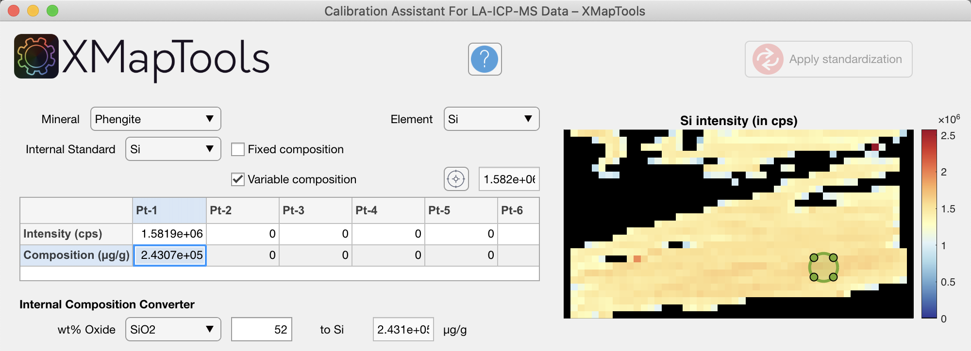
Figure 2: Example of internal calibration of phengite using Si as internal standard and a variable reference composition. A value of SiO2 = 52 wt% is assigned to the phengite core (Pt-1).
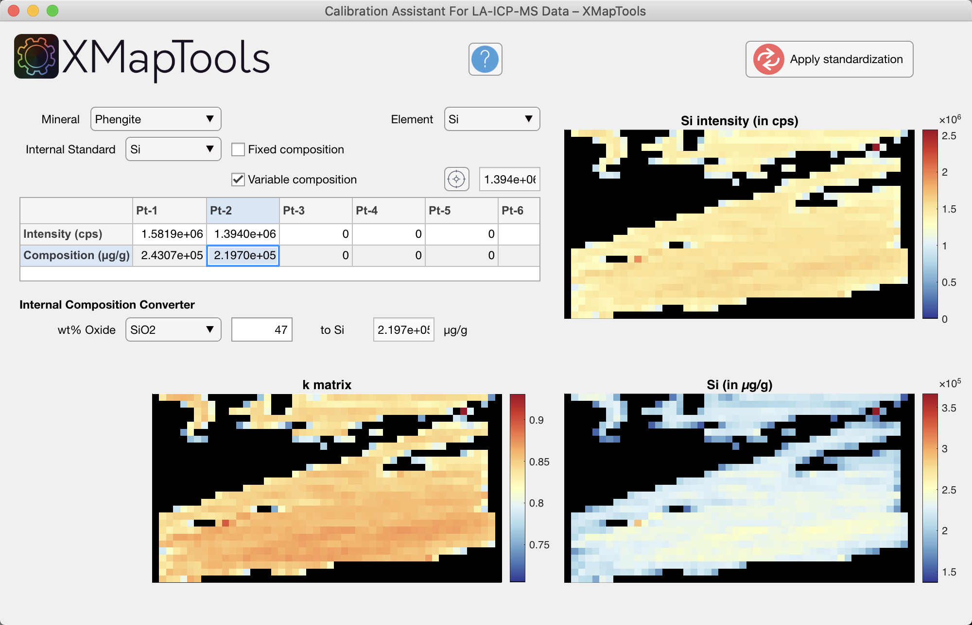
Figure 3: Example with a value of SiO2 = 47 wt% assigned to the muscovite rim (Pt-2). Two maps are shown below: the k-matrix calculated using the internal standard with variable composition and the calibrated map for Si expressed in µg/g. Note that compared to Figure 1, Si is not homogeneous throughout the mica.
Press the Apply Standardisation button to generate the compositional maps available in the Quantity category of the Primary Menu. The maps are expressed in µg/g of elements. You can convert them to wt% of oxides using the internal converter: right-click on a Quanti file and select Convert.
TIP
After converting the maps, the name of the maps can be changed (this is not done by the converter).
Generate spider plots
The button Spider (Open Spider Module) opens the module Spider Plot. This button is only available when a quanti file or any map within a quanti file is selected in the primary menu.
For more detailed information on the Spider Module, see the dedicated Spider Module page.