XMapTools documentation for EPMA

Table of contents

EPMA & SEM:

• Data compatibility (EPMA)
  • CAMECA
    • Maps
    • Spot analyses
• Data conversion
  • EPMA converter module
• Generation of mosaics
  • Grid mosaic
  • Real mosaic
• Importing data
• Importing calibrated data (EPMA & SEM)
  • Step 1: Adding calibrated maps
  • Step 2: Data conversion (optional)
  • Step 3: Classification of quantitative data
  • Step 4: Splitting a merged dataset
• Classification
  • Classification parameters & algorithms
  • Training and classification
  • Filtering options
  • Mask analysis & visualisation
• Calibration (EPMA)
  • Standard data
  • Map calibration
  • Calibration assistant (EPMA)
  • Local bulk compositions

Data compatibility for EPMA

CAMECA microprobes

CAMECA Maps

Because of the file format used by CAMECA, XMapTools is reading the information of the following lines in the header:

• Start [map coordinates]
• Step Number [number of columns]
• Line Number [Number of rows]
• Image [to detect the map name].
• If the number of steps and rows doesn't match the size of the table, data won't be imported. The file name is not used to determine the element name when Image is defined.

Therefore the minimum number of header lines is:

Start :  X = 15702 Y = -24236 Z = 240
Step Number : 416
Line Number : 440

Y Unit : cts
Image  : Ca Ka

[Data table should start here... use tabulation, no coma]

XMapTools can import two types of map data file that are generated by CAMECA microprobes.

Type 1: Simple

FileName :   Bustamante 18-1-2013.impDat (Current dataset : 4) 
Signal(s) Used :  Vs1 BSE Z, Na Ka, Ca Ka, Fe Ka, Mg Ka, Al Ka, Si Ka Eds, S  Ka Eds, Cl Ka Eds, K  Ka Eds, Ti Ka Eds, Mn Ka Eds, Zr La Eds, Ba La Eds 
Spectromers Conditions :   Sp1 LTAP,  Sp2 LPET,  Sp3 LLIF,  Sp4 LTAP,  Sp5 LTAP,  Eds 1,  Eds 2,  Eds 3,  Eds 4,  Eds 5,  Eds 6,  Eds 7,  Eds 8 
Full Spectromers Conditions :   Sp1 LTAP(2d= 25.745,K= 0.00218),  Sp2 LPET(2d= 8.75,K= 0.000144),  Sp3 LLIF(2d= 4.0267,K= 0.000058),  Sp4 LTAP(2d= 25.745,K= 0.00218),  Sp5 LTAP(2d= 25.745,K= 0.00218),  Eds 1,  Eds 2,  Eds 3,  Eds 4,  Eds 5,  Eds 6,  Eds 7,  Eds 8 
Column Conditions :  Cond 1 : 15.1keV 302.5757nA  
Date :  19-Jan-2013 
User Name :  sx 
Setup Name :  Bustamante.impSet 
DataSet Comment :   
Comment :   
Analysis Date :  1/18/2013 12:42:21 PM 
Project Name :  Caetano 
Sample Name :  2013-01-18 
Pha Parameters :  	 
 		Bias	Gain	Dtime	Blin	Wind	Mode	 
  Sp1(Na Ka)	1300	2635	3	560	 	Inte	 
  Sp2(Ca Ka)	1289	1100	3	560	 	Inte	 
  Sp3(Fe Ka)	1824	550	3	560	 	Inte	 
  Sp4(Mg Ka)	1293	2964	3	560	 	Inte	 
  Sp5(Al Ka)	1280	2943	3	560	 	Inte 
 EDS: Si Ka 
 EDS: S  Ka 
 EDS: Cl Ka 
 EDS: K  Ka 
 EDS: Ti Ka 
 EDS: Mn Ka 
 EDS: Zr La 
 EDS: Ba La 
Peak Position :   Sp1 46363,  Sp2 38388,  Sp3 48084,  Sp4 38500,  Sp5 32460 
Start :   X = 7386 Y = -17430 Z = 49 
Stop :   
Dwell Time :  0.03 Sec  
Acquisition type :   Stage Grid  
Step Number :  1001 
Line Number :  614 
Beam Size :  3 µm 
Step Size :  4. 

Y Unit : 
Image  : BSE Z

83.0000	83.0000	88.0000	82.0000	82.0000	81.0000	82.0000	83.0000	83.0000	84.0000	89.0000	92.0000	83.0000	87.0000	83.0000	85.0000	86.0000	86.0000	85.0000	86.0000	88.0000	85.0000	82.0000	87.0000	85.0000	84.0000	87.0000	87.0000	85.0000	85.0000	85.0000	87.0000	86.0000	86.0000	85.0000	86.0000	90.0000	87.0000	87.0000	87.0000	86.0000	96.0000	107.0000	89.0000	88.0000	90.0000	101.0000	113.0000	92.0000	101.0000	81.0000	96.0000	79.0000	81.0000	91.0000	82.0000	128.0000	135.0000	126.0000	120.0000	94.0000	112.0000	84.0000	80.0000	82.0000	83.0000	88.0000	97.0000	82.0000	81.0000	80.0000	81.0000	82.0000	81.0000	131.0000	97.0000	82.0000	83.0000	84.0000	84.0000	80.0000	80.0000	81.0000	87.0000	96.0000	83.0000	84.0000	85.0000	79.0000	82.0000	81.0000	80.0000	81.0000	80.0000	80.0000	79.0000	80.0000	83.0000	82.0000	82.0000	82.0000	82.0000	80.0000	80.0000	86.0000	82.0000	86.0000	85.0000	81.0000	84.0000	83.0000	84.0000	85.0000	83.0000	82.0000	79.0000	81.0000	80.0000	83.0000	84.0000	84.0000	83.0000	84.0000	84.0000	80.0000	80.0000	80.0000	81.0000	85.0000	85.0000	85.0000	83.0000	84.0000	82.0000	83.0000	87.0000	87.0000	84.0000	80.0000	81.0000	85.0000	85.0000	84.0000	83.0000	85.0000	92.0000	81.0000	83.0000	85.0000	85.0000	84.0000	84.0000	84.0000	85.0000	87.0000	87.0000	85.0000	84.0000	84.0000	81.0000	85.0000	80.0000	84.0000	83.0000	84.0000	83.0000	89.0000	91.0000	88.0000	85.0000	89.0000	91.0000	95.0000	91.0000	96.0000	82.0000	84.0000	83.0000	82.0000	86.0000	82.0000	79.0000	86.0000	84.0000	83.0000	83.0000	83.0000	84.0000	83.0000	83.0000	84.0000	84.0000	80.0000	86.0000	86.0000	83.0000	85.0000	83.0000	83.0000	82.0000	91.0000	79.0000	80.0000	76.0000	82.0000	81.0000	81.0000	81.0000	81.0000	81.0000	80.0000	81.0000	83.0000	85.0000	85.0000	86.0000	87.0000	81.0000	83.0000	83.0000	79.0000	80.0000	81.0000	78.0000	84.0000	83.0000	83.0000	76.0000	78.0000	81.0000	80.0000	80.0000	81.0000	80.0000	81.0000	75.0000	81.0000	80.0000	86.0000	115.0000	78.0000	80.0000	83.0000	79.0000	104.0000	102.0000	94.0000	90.0000	84.0000	84.0000	82.0000	84.0000	82.0000	81.0000	81.0000	82.0000	82.0000	83.0000	83.0000	83.0000	83.0000	80.0000	87.0000	98.0000	85.0000	79.0000	82.0000	82.0000	82.0000	83.0000	79.0000	100.0000	115.0000	80.0000	80.0000	80.0000	81.0000	90.0000	75.0000	82.0000	80.0000	79.0000	78.0000	84.0000	81.0000	81.0000	111.0000	107.0000	83.0000	85.0000	83.0000	82.0000	111.0000	84.0000	80.0000	83.0000	70.0000	80.0000	82.0000	83.0000	82.0000	82.0000	81.0000	92.0000	83.0000	86.0000	85.0000	102.0000	101.0000	79.0000	87.0000	84.0000	84.0000	82.0000	86.0000	95.0000	124.0000	84.0000	82.0000	80.0000	85.0000	85.0000	80.0000	81.0000	88.0000	92.0000	88.0000	86.0000	76.0000	83.0000	86.0000	82.0000	82.0000	83.0000	80.0000	80.0000	79.0000	80.0000	80.0000	78.0000	82.0000	88.0000	89.0000	91.0000	88.0000	86.0000	92.0000	97.0000	81.0000	78.0000	79.0000	79.0000	82.0000	82.0000	80.0000	77.0000	80.0000	79.0000	79.0000	80.0000	87.0000	85.0000	85.0000	85.0000	84.0000	83.0000	80.0000	80.0000	79.0000	79.0000	78.0000	84.0000	82.0000	81.0000	80.0000	78.0000	79.0000	80.0000	83.0000	79.0000	81.0000	80.0000	79.0000	77.0000	77.0000	78.0000	85.0000	85.0000	82.0000	85.0000	79.0000	80.0000	80.0000	79.0000	79.0000	79.0000	79.0000	80.0000	85.0000	84.0000	82.0000	80.0000	80.0000	79.0000	79.0000	80.0000	79.0000	80.0000	80.0000	79.0000	80.0000	80.0000	80.0000	82.0000	85.0000	85.0000	85.0000	85.0000	87.0000	80.0000	80.0000	80.0000	84.0000	81.0000	81.0000	94.0000	81.0000	81.0000	81.0000	89.0000	81.0000	80.0000	79.0000	80.0000	85.0000	85.0000	83.0000	84.0000	85.0000	80.0000	80.0000	83.0000	85.0000	88.0000	86.0000	80.0000	80.0000	80.0000	80.0000	80.0000	80.0000	80.0000	81.0000	82.0000	80.0000	83.0000	84.0000	122.0000	99.0000	76.0000	80.0000	82.0000	83.0000	82.0000	86.0000	80.0000	75.0000	91.0000	87.0000	61.0000	74.0000	59.0000	82.0000	94.0000	85.0000	105.0000	87.0000	52.0000	82.0000	88.0000	84.0000	79.0000	80.0000	80.0000	79.0000	80.0000	79.0000	79.0000	81.0000	85.0000	84.0000	84.0000	85.0000	86.0000	85.0000	85.0000	79.0000	80.0000	79.0000	83.0000	80.0000	79.0000	79.0000	79.0000	89.0000	78.0000	80.0000	80.0000	79.0000	79.0000	80.0000	80.0000	81.0000	85.0000	79.0000	78.0000	85.0000	82.0000	78.0000	79.0000	79.0000	78.0000	80.0000	78.0000	78.0000	78.0000	78.0000	79.0000	78.0000	78.0000	78.0000	78.0000	79.0000	79.0000	78.0000	84.0000	85.0000	84.0000	79.0000	79.0000	79.0000	88.0000	83.0000	79.0000	86.0000	98.0000	85.0000	81.0000	80.0000	79.0000	83.0000	79.0000	79.0000	83.0000	85.0000	84.0000	77.0000	77.0000	80.0000	81.0000	79.0000	81.0000	78.0000	78.0000	78.0000	79.0000	78.0000	78.0000	79.0000	79.0000	79.0000	79.0000	86.0000	84.0000	80.0000	79.0000	79.0000	82.0000	80.0000	79.0000	79.0000	78.0000	78.0000	79.0000	79.0000	78.0000	78.0000	79.0000	80.0000	78.0000	85.0000	77.0000	76.0000	78.0000	78.0000	77.0000	76.0000	79.0000	78.0000	79.0000	78.0000	79.0000	84.0000	85.0000	84.0000	85.0000	84.0000	81.0000	85.0000	84.0000	78.0000	78.0000	79.0000	79.0000	78.0000	79.0000	80.0000	80.0000	112.0000	86.0000	88.0000	86.0000	86.0000	84.0000	83.0000	83.0000	84.0000	83.0000	84.0000	76.0000	79.0000	79.0000	78.0000	78.0000	79.0000	79.0000	79.0000	79.0000	79.0000	79.0000	82.0000	89.0000	88.0000	85.0000	85.0000	86.0000	85.0000	84.0000	85.0000	83.0000	85.0000	85.0000	83.0000	89.0000	86.0000	84.0000	86.0000	87.0000	85.0000	86.0000	85.0000	84.0000	87.0000	88.0000	88.0000	85.0000	80.0000	80.0000	80.0000	79.0000	78.0000	79.0000	79.0000	79.0000	80.0000	79.0000	81.0000	86.0000	85.0000	86.0000	86.0000	84.0000	85.0000	84.0000	84.0000	84.0000	91.0000	85.0000	84.0000	83.0000	83.0000	86.0000	88.0000	89.0000	88.0000	86.0000	85.0000	83.0000	84.0000	84.0000	84.0000	84.0000	83.0000	89.0000	79.0000	78.0000	84.0000	81.0000	84.0000	84.0000	83.0000	80.0000	86.0000	83.0000	81.0000	81.0000	80.0000	78.0000	78.0000	81.0000	78.0000	79.0000	123.0000	107.0000	82.0000	83.0000	78.0000	76.0000	78.0000	77.0000	78.0000	78.0000	81.0000	80.0000	75.0000	77.0000	78.0000	78.0000	84.0000	78.0000	79.0000	79.0000	85.0000	85.0000	84.0000	82.0000	84.0000	85.0000	81.0000	85.0000	83.0000	84.0000	84.0000	84.0000	84.0000	84.0000	85.0000	84.0000	85.0000	84.0000	84.0000	84.0000	85.0000	85.0000	90.0000	86.0000	92.0000	86.0000	85.0000	85.0000	85.0000	86.0000	106.0000	84.0000	83.0000	85.0000	85.0000	84.0000	87.0000	108.0000	84.0000	83.0000	84.0000	84.0000	84.0000	88.0000	83.0000	83.0000	83.0000	84.0000	83.0000	85.0000	94.0000	84.0000	85.0000	85.0000	79.0000	78.0000	78.0000	78.0000	78.0000	79.0000	79.0000	79.0000	79.0000	81.0000	86.0000	117.0000	85.0000	84.0000	85.0000	85.0000	83.0000	105.0000	86.0000	86.0000	89.0000	89.0000	88.0000	89.0000	90.0000	84.0000	84.0000	83.0000	77.0000	76.0000	80.0000	82.0000	79.0000	82.0000	88.0000	82.0000	84.0000	83.0000	92.0000	88.0000	78.0000	78.0000	77.0000	78.0000	78.0000	77.0000	80.0000	80.0000	77.0000	77.0000	77.0000	77.0000	77.0000	82.0000	96.0000	83.0000	83.0000	77.0000	77.0000	77.0000	78.0000	77.0000	78.0000	78.0000	78.0000	84.0000	83.0000	84.0000	84.0000	84.0000	84.0000	83.0000	84.0000	84.0000	83.0000	83.0000	84.0000	82.0000	82.0000	83.0000	83.0000	87.0000	82.0000	77.0000	85.0000	76.0000	77.0000	77.0000	78.0000	78.0000	77.0000	77.0000	78.0000	83.0000	84.0000	84.0000	85.0000	82.0000	82.0000	83.0000	82.0000	82.0000	82.0000	83.0000	86.0000	81.0000	82.0000	84.0000	83.0000	83.0000	83.0000	83.0000	77.0000	77.0000	78.0000	77.0000	76.0000	77.0000	79.0000	80.0000	90.0000	83.0000	82.0000	82.0000	82.0000	82.0000	83.0000	85.0000	87.0000	84.0000	82.0000	90.0000	83.0000	89.0000	82.0000	81.0000	83.0000	83.0000	83.0000	83.0000	83.0000	82.0000	80.0000	77.0000	83.0000	82.0000	82.0000	82.0000	83.0000	82.0000	82.0000	82.0000	78.0000	77.0000	77.0000	77.0000	77.0000	77.0000	77.0000	78.0000	78.0000	88.0000	82.0000	82.0000	83.0000	83.0000	84.0000	83.0000	77.0000	77.0000	77.0000	77.0000	77.0000	77.0000	77.0000	82.0000	76.0000	77.0000	79.0000	76.0000	77.0000	78.0000	76.0000	76.0000	77.0000	76.0000	77.0000	77.0000	74.0000	74.0000	77.0000	77.0000	77.0000	77.0000	76.0000	76.0000	77.0000	77.0000	77.0000	76.0000	77.0000	77.0000	76.0000	77.0000	78.0000
82.0000	83.0000	82.0000	80.0000	79.0000	80.0000	84.0000	81.0000	81.0000	82.0000	85.0000	88.0000	86.0000	86.0000	84.0000	83.0000	83.0000	84.0000	83.0000	84.0000	83.0000	85.0000	85.0000	87.0000	86.0000	84.0000	91.0000	91.0000	85.0000	85.0000	85.0000	86.0000	87.0000	89.0000	91.0000	87.0000	94.0000	85.0000	86.0000	90.0000	128.0000	95.0000	110.0000	115.0000	105.0000	105.0000	93.0000	95.0000	102.0000	78.0000	87.0000	85.0000	80.0000	80.0000	88.0000	80.0000	84.0000	128.0000	112.0000	113.0000	102.0000	126.0000	80.0000	80.0000	80.0000	83.0000	85.0000	82.0000	77.0000	79.0000	79.0000	81.0000	81.0000	81.0000	97.0000	90.0000	81.0000	82.0000	83.0000	82.0000	79.0000	82.0000	82.0000	84.0000	87.0000	82.0000	82.0000	84.0000	77.0000	85.0000	80.0000	80.0000	79.0000	80.0000	79.0000	79.0000	82.0000	82.0000	82.0000	81.0000	81.0000	81.0000	81.0000	81.0000	84.0000	82.0000	82.0000	79.0000	79.0000	81.0000	83.0000	83.0000	84.0000	82.0000	78.0000	78.0000	81.0000	80.0000	84.0000	83.0000	83.0000	82.0000	83.0000	81.0000	79.0000	79.0000	79.0000	79.0000	83.0000	83.0000	83.0000	85.0000	85.0000	80.0000	82.0000	84.0000	84.0000	82.0000	81.0000	83.0000	82.0000	83.0000	83.0000	80.0000	83.0000	82.0000	85.0000	83.0000	79.0000	82.0000	83.0000	83.0000	82.0000	85.0000	86.0000	87.0000	84.0000	84.0000	82.0000	82.0000	83.0000	82.0000	81.0000	83.0000	84.0000	84.0000	89.0000	90.0000	81.0000	87.0000	90.0000	89.0000	90.0000	94.0000	89.0000	81.0000	82.0000	82.0000	80.0000	80.0000	84.0000	79.0000	83.0000	82.0000	82.0000	82.0000	82.0000	83.0000	81.0000	95.0000	84.0000	82.0000	83.0000	86.0000	92.0000	84.0000	81.0000	82.0000	82.0000	81.0000	88.0000	78.0000	80.0000	79.0000	81.0000	80.0000	80.0000	80.0000	81.0000	80.0000	80.0000	82.0000	82.0000	79.0000	82.0000	78.0000	83.0000	80.0000	82.0000	83.0000	78.0000	81.0000	80.0000	83.0000	82.0000	82.0000	84.0000	76.0000	78.0000	79.0000	79.0000	80.0000	81.0000	79.0000	80.0000	80.0000	79.0000	80.0000	82.0000	123.0000	88.0000	78.0000	81.0000	75.0000	89.0000	84.0000	90.0000	87.0000	82.0000	160.0000	105.0000	97.0000	82.0000	79.0000	82.0000	81.0000	82.0000	81.0000	82.0000	81.0000	82.0000	75.0000	89.0000	85.0000	83.0000	79.0000	80.0000	81.0000	80.0000	81.0000	82.0000	105.0000	93.0000	79.0000	80.0000	80.0000	80.0000	106.0000	81.0000	77.0000	79.0000	78.0000	83.0000	82.0000	80.0000	82.0000	125.0000	84.0000	83.0000	81.0000	87.0000	81.0000	73.0000	82.0000	82.0000	83.0000	91.0000	81.0000	80.0000	80.0000	81.0000	81.0000	81.0000	87.0000	82.0000	84.0000	82.0000	92.0000	79.0000	78.0000	83.0000	84.0000	82.0000	81.0000	82.0000	87.0000	92.0000	79.0000	79.0000	81.0000	87.0000	79.0000	83.0000	83.0000	86.0000	89.0000	91.0000	79.0000	78.0000	90.0000	78.0000	77.0000	78.0000	83.0000	80.0000	79.0000	79.0000	79.0000	84.0000	79.0000	80.0000	81.0000	83.0000	87.0000	82.0000	79.0000	80.0000	89.0000	81.0000	77.0000	77.0000	80.0000	79.0000	78.0000	80.0000	80.0000	80.0000	78.0000	76.0000	79.0000	82.0000	84.0000	85.0000	84.0000	83.0000	78.0000	78.0000	79.0000	79.0000	79.0000	80.0000	79.0000	78.0000	80.0000	76.0000	77.0000	78.0000	79.0000	79.0000	91.0000	81.0000	79.0000	81.0000	81.0000	82.0000	82.0000	84.0000	84.0000	81.0000	79.0000	82.0000	77.0000	80.0000	80.0000	82.0000	78.0000	78.0000	78.0000	92.0000	81.0000	85.0000	78.0000	84.0000	77.0000	79.0000	79.0000	78.0000	79.0000	79.0000	78.0000	79.0000	86.0000	79.0000	86.0000	84.0000	84.0000	85.0000	85.0000	90.0000	80.0000	79.0000	79.0000	83.0000	80.0000	80.0000	84.0000	79.0000	80.0000	131.0000	91.0000	83.0000	79.0000	80.0000	82.0000	82.0000	85.0000	80.0000	80.0000	80.0000	79.0000	80.0000	81.0000	84.0000	88.0000	86.0000	80.0000	80.0000	80.0000	80.0000	80.0000	79.0000	80.0000	80.0000	81.0000	81.0000	83.0000	86.0000	103.0000	86.0000	82.0000	81.0000	85.0000	88.0000	85.0000	83.0000	86.0000	59.0000	101.0000	91.0000	57.0000	58.0000	66.0000	61.0000	60.0000	102.0000	87.0000	80.0000	56.0000	90.0000	92.0000	85.0000	81.0000	80.0000	80.0000	81.0000	81.0000	79.0000	78.0000	79.0000	86.0000	84.0000	83.0000	83.0000	84.0000	85.0000	84.0000	78.0000	78.0000	78.0000	85.0000	84.0000	79.0000	78.0000	78.0000	79.0000	78.0000	79.0000	79.0000	78.0000	79.0000	78.0000	79.0000	79.0000	84.0000	85.0000	78.0000	84.0000	84.0000	77.0000	78.0000	78.0000	78.0000	76.0000	75.0000	74.0000	76.0000	78.0000	78.0000	77.0000	75.0000	75.0000	81.0000	78.0000	78.0000	77.0000	83.0000	82.0000	82.0000	77.0000	78.0000	77.0000	83.0000	77.0000	78.0000	84.0000	104.0000	84.0000	75.0000	76.0000	78.0000	82.0000	78.0000	79.0000	83.0000	83.0000	84.0000	78.0000	78.0000	78.0000	75.0000	76.0000	76.0000	77.0000	77.0000	77.0000	77.0000	76.0000	77.0000	78.0000	78.0000	80.0000	85.0000	83.0000	84.0000	79.0000	78.0000	78.0000	75.0000	79.0000	78.0000	78.0000	77.0000	77.0000	78.0000	78.0000	78.0000	77.0000	78.0000	77.0000	77.0000	81.0000	77.0000	75.0000	78.0000	78.0000	77.0000	80.0000	79.0000	78.0000	78.0000	77.0000	80.0000	83.0000	84.0000	84.0000	83.0000	105.0000	84.0000	89.0000	83.0000	76.0000	77.0000	77.0000	78.0000	77.0000	79.0000	79.0000	79.0000	146.0000	87.0000	89.0000	84.0000	85.0000	83.0000	83.0000	82.0000	82.0000	83.0000	81.0000	78.0000	76.0000	78.0000	78.0000	77.0000	78.0000	78.0000	78.0000	78.0000	79.0000	79.0000	81.0000	81.0000	82.0000	83.0000	85.0000	85.0000	82.0000	84.0000	84.0000	84.0000	84.0000	85.0000	83.0000	83.0000	80.0000	86.0000	90.0000	88.0000	82.0000	85.0000	85.0000	85.0000	86.0000	85.0000	84.0000	84.0000	82.0000	79.0000	78.0000	78.0000	78.0000	78.0000	78.0000	79.0000	79.0000	85.0000	81.0000	85.0000	85.0000	85.0000	85.0000	83.0000	85.0000	84.0000	83.0000	84.0000	83.0000	84.0000	83.0000	83.0000	84.0000	93.0000	87.0000	85.0000	83.0000	85.0000	83.0000	83.0000	82.0000	87.0000	85.0000	91.0000	85.0000	85.0000	77.0000	78.0000	82.0000	79.0000	81.0000	82.0000	110.0000	77.0000	76.0000	76.0000	77.0000	79.0000	78.0000	78.0000	78.0000	78.0000	78.0000	77.0000	81.0000	102.0000	78.0000	77.0000	77.0000	77.0000	78.0000	77.0000	76.0000	78.0000	77.0000	79.0000	78.0000	77.0000	78.0000	78.0000	76.0000	76.0000	78.0000	78.0000	83.0000	84.0000	79.0000	82.0000	84.0000	84.0000	83.0000	83.0000	84.0000	83.0000	84.0000	84.0000	84.0000	85.0000	83.0000	86.0000	90.0000	83.0000	83.0000	84.0000	85.0000	84.0000	84.0000	83.0000	84.0000	85.0000	85.0000	84.0000	84.0000	95.0000	102.0000	83.0000	83.0000	84.0000	84.0000	82.0000	83.0000	95.0000	83.0000	83.0000	83.0000	89.0000	83.0000	83.0000	82.0000	83.0000	83.0000	82.0000	83.0000	82.0000	85.0000	82.0000	83.0000	83.0000	78.0000	78.0000	77.0000	77.0000	78.0000	78.0000	78.0000	78.0000	78.0000	81.0000	90.0000	89.0000	83.0000	85.0000	85.0000	96.0000	116.0000	101.0000	84.0000	80.0000	90.0000	86.0000	88.0000	87.0000	87.0000	82.0000	82.0000	78.0000	77.0000	88.0000	78.0000	77.0000	76.0000	79.0000	84.0000	82.0000	83.0000	83.0000	81.0000	77.0000	76.0000	76.0000	76.0000	76.0000	76.0000	76.0000	88.0000	76.0000	76.0000	77.0000	76.0000	77.0000	76.0000	81.0000	83.0000	85.0000	80.0000	76.0000	77.0000	76.0000	77.0000	76.0000	77.0000	77.0000	78.0000	82.0000	82.0000	83.0000	84.0000	85.0000	83.0000	82.0000	82.0000	82.0000	81.0000	84.0000	83.0000	82.0000	81.0000	82.0000	82.0000	83.0000	82.0000	81.0000	77.0000	78.0000	76.0000	76.0000	77.0000	77.0000	76.0000	77.0000	82.0000	80.0000	82.0000	83.0000	83.0000	82.0000	81.0000	80.0000	82.0000	82.0000	82.0000	81.0000	84.0000	81.0000	82.0000	83.0000	80.0000	80.0000	82.0000	76.0000	76.0000	76.0000	77.0000	77.0000	76.0000	77.0000	78.0000	76.0000	79.0000	82.0000	82.0000	82.0000	82.0000	82.0000	88.0000	85.0000	86.0000	82.0000	82.0000	107.0000	83.0000	85.0000	80.0000	78.0000	83.0000	82.0000	85.0000	81.0000	82.0000	81.0000	78.0000	76.0000	83.0000	82.0000	80.0000	80.0000	81.0000	81.0000	82.0000	81.0000	74.0000	76.0000	76.0000	77.0000	77.0000	76.0000	76.0000	78.0000	77.0000	77.0000	81.0000	82.0000	82.0000	92.0000	83.0000	82.0000	76.0000	79.0000	76.0000	77.0000	77.0000	76.0000	77.0000	81.0000	77.0000	77.0000	80.0000	76.0000	76.0000	76.0000	76.0000	76.0000	76.0000	76.0000	76.0000	76.0000	76.0000	76.0000	76.0000	76.0000	76.0000	76.0000	76.0000	76.0000	76.0000	76.0000	76.0000	76.0000	77.0000	76.0000	76.0000	77.0000	77.0000

Type 2: With column and row numbers

FileName :  Celine_091321.impDat (Current dataset : 1)
Signal(s) Used : Ca Ka, Na Ka, K  Ka, Al Ka, Mn Ka, Cr Ka, Mg Ka, Ti Ka, Si Ka, Fe Ka
Spectrometers Conditions :  Sp1 PET,  Sp2 LTAP,  Sp3 LPET,  Sp4 TAP,  Sp5 LLIF,  Sp1 PET,  Sp2 LTAP,  Sp3 LPET,  Sp4 TAP,  Sp5 LLIF
Full Spectrometers Conditions :  Sp1 PET(2d= 8.75,K= 0.000144),  Sp2 LTAP(2d= 25.745,K= 0.00218),  Sp3 LPET(2d= 8.75,K= 0.000144),  Sp4 TAP(2d= 25.745,K= 0.00218),  Sp5 LLIF(2d= 4.0267,K= 5.8E-05),  Sp1 PET(2d= 8.75,K= 0.000144),  Sp2 LTAP(2d= 25.745,K= 0.00218),  Sp3 LPET(2d= 8.75,K= 0.000144),  Sp4 TAP(2d= 25.745,K= 0.00218),  Sp5 LLIF(2d= 4.0267,K= 5.8E-05)
Column Conditions : Cond 1 : 15keV 278.8476nA , Cond 2 : 15keV 280.8923nA 
	, Cond 1 : Ca Ka, Na Ka, K  Ka, Al Ka, Mn Ka
	, Cond 2 : Cr Ka, Mg Ka, Ti Ka, Si Ka, Fe Ka
Date : Sep-15-2021
User Name : SX-663\SX-User
Setup Name : C:\SX data\Analysis Setups\Image&Profiles\Celine_091321.impSet
DataSet Comment : BOO17-5N_Map1
Comment :  
Analysis Date : Tuesday, September 14, 2021 6:57:42 AM
Project Name : Default Project
Sample Name : Default Sample
Analysis Parameters : 	
Sp	Elements	Xtal	Position	Bias	Gain	Dtime	Blin	Wind	Mode	
Sp1	Ca Ka		PET	38388	1304	1031	3	560	 	Inte
Sp2	Na Ka		LTAP	46363	1311	3055	3	560	 	Inte
Sp3	K  Ka		LPET	42765	1846	985	3	560	 	Inte
Sp4	Al Ka		TAP	32459	1325	3181	3	560	 	Inte
Sp5	Mn Ka		LLIF	52202	1820	411	3	560	 	Inte
Sp1	Cr Ka		PET	26172	1304	1031	3	560	 	Inte
Sp2	Mg Ka		LTAP	38500	1311	3055	3	560	 	Inte
Sp3	Ti Ka		LPET	31416	1846	985	3	560	 	Inte
Sp4	Si Ka		TAP	27737	1325	3181	3	560	 	Inte
Sp5	Fe Ka		LLIF	48083	1820	411	3	560	 	Inte
Peak Position :  Sp1 38388,  Sp2 46363,  Sp3 42765,  Sp4 32459,  Sp5 52202,  Sp1 26172,  Sp2 38500,  Sp3 31416,  Sp4 27737,  Sp5 48083
Start :  X = -1748 Y = -29677 Z = 14
Stop : 
Dwell Time : 0.07 Sec 
Acquisition type :  Stage Grid 
Step Number : 504
Line Number : 504
Beam Size : N/A
Step Size : 4.000



Y Unit : cts


	1	2	3	4	5	6	7	8	9	10	11	12	13	14	15	16	17	18	19	20	21	22	23	24	25	26	27	28	29	30	31	32	33	34	35	36	37	38	39	40	41	42	43	44	45	46	47	48	49	50	51	52	53	54	55	56	57	58	59	60	61	62	63	64	65	66	67	68	69	70	71	72	73	74	75	76	77	78	79	80	81	82	83	84	85	86	87	88	89	90	91	92	93	94	95	96	97	98	99	100	101	102	103	104	105	106	107	108	109	110	111	112	113	114	115	116	117	118	119	120	121	122	123	124	125	126	127	128	129	130	131	132	133	134	135	136	137	138	139	140	141	142	143	144	145	146	147	148	149	150	151	152	153	154	155	156	157	158	159	160	161	162	163	164	165	166	167	168	169	170	171	172	173	174	175	176	177	178	179	180	181	182	183	184	185	186	187	188	189	190	191	192	193	194	195	196	197	198	199	200	201	202	203	204	205	206	207	208	209	210	211	212	213	214	215	216	217	218	219	220	221	222	223	224	225	226	227	228	229	230	231	232	233	234	235	236	237	238	239	240	241	242	243	244	245	246	247	248	249	250	251	252	253	254	255	256	257	258	259	260	261	262	263	264	265	266	267	268	269	270	271	272	273	274	275	276	277	278	279	280	281	282	283	284	285	286	287	288	289	290	291	292	293	294	295	296	297	298	299	300	301	302	303	304	305	306	307	308	309	310	311	312	313	314	315	316	317	318	319	320	321	322	323	324	325	326	327	328	329	330	331	332	333	334	335	336	337	338	339	340	341	342	343	344	345	346	347	348	349	350	351	352	353	354	355	356	357	358	359	360	361	362	363	364	365	366	367	368	369	370	371	372	373	374	375	376	377	378	379	380	381	382	383	384	385	386	387	388	389	390	391	392	393	394	395	396	397	398	399	400	401	402	403	404	405	406	407	408	409	410	411	412	413	414	415	416	417	418	419	420	421	422	423	424	425	426	427	428	429	430	431	432	433	434	435	436	437	438	439	440	441	442	443	444	445	446	447	448	449	450	451	452	453	454	455	456	457	458	459	460	461	462	463	464	465	466	467	468	469	470	471	472	473	474	475	476	477	478	479	480	481	482	483	484	485	486	487	488	489	490	491	492	493	494	495	496	497	498	499	500	501	502	503	504
1	1987	1954	2079	1974	2083	2103	2073	2128	2028	1850	2121	1916	1938	2013	2066	2037	2109	2075	2093	2032	2053	2087	2118	2130	2082	2047	1986	2056	1994	2006	1920	1949	1970	1981	1922	2279	1986	1984	1992	1983	1960	1958	1996	1910	1972	1939	1934	1962	1984	1948	1933	1929	1850	1921	1948	1941	1942	1978	1997	2014	1973	1939	1985	1871	1595	1935	1964	1864	1905	1894	1896	1836	1894	1908	1920	1804	1876	1871	1812	1833	1928	1830	1844	1874	1982	1853	1934	1857	1920	1837	1856	1882	1964	2920	2025	1817	1908	1967	1925	1901	1947	1895	1912	1886	1967	1898	1945	1939	1935	1975	1962	2007	1963	1930	1941	1914	1893	1994	1986	1930	1954	2039	1950	2004	2005	1976	1943	1906	2046	2070	2105	2129	2971	2420	2304	2475	2051	2036	2184	2213	2047	2049	2064	2043	2788	2104	1979	1972	2056	2022	2153	2087	2180	2124	2094	1993	1992	2097	1957	2016	2014	3758	2197	2042	2032	2024	2018	2226	2570	3155	2870	2174	2000	1983	1942	2018	1974	1944	2043	1962	2047	1954	1961	2035	2083	2085	2003	2020	2069	2153	1988	1957	2014	2087	2054	1963	2052	2043	1999	1947	2007	2109	2035	2016	2100	2000	2013	1980	2012	2051	2072	2083	1978	2015	2078	2232	3343	3864	3847	2105	3254	3823	3869	3952	4521	3751	4286	4042	3589	3693	3570	3397	3597	3553	3877	3837	3747	3997	3824	2952	2986	3676	3975	4050	4008	3699	3649	3843	3940	4099	3524	3987	4367	3461	2725	2960	2424	2145	2095	2132	1941	2070	2081	2488	2146	2270	2069	2080	2078	2062	2666	2099	2120	2152	2076	2052	2041	2033	2054	2067	2222	2012	2114	2088	2031	2142	2107	2265	2502	2852	3239	3536	3372	3914	2630	3431	3709	2810	3996	3249	3964	2999	3846	3832	3698	3362	2881	2706	2166	1969	1923	2051	2080	2138	2002	2054	2021	1992	2047	1967	2025	2007	1934	2068	1980	1990	1914	2039	1982	1995	2016	2098	2067	2048	1999	2044	3706	3266	1668	1885	1802	2099	1990	2050	1939	2059	2032	2039	2112	2146	2052	2088	2062	2041	2006	2086	2084	2090	2087	2046	1996	2078	2103	2030	2069	2018	2019	1994	1957	2042	1978	2160	2823	3063	2137	2088	2327	1857	2111	2065	2149	2063	2049	1962	1987	2056	2027	2041	1925	1945	2027	2001	1985	2006	2000	2033	1998	1951	1929	1985	1983	1939	1983	1967	1990	2063	1946	2017	1998	1990	2039	2048	2012	1996	2065	2041	2001	2053	2022	2013	1974	2074	2572	2105	2021	2040	2064	2071	2022	2020	2057	2032	2056	2095	1877	2073	1991	1990	2428	1931	2029	2031	2016	2006	2046	2024	1984	1941	2071	2061	2049	2042	1974	2010	1989	1970	2000	1984	2010	2001	1932	1921	1949	1958	2033	2998	1998	2039	2012	2023	1988	2020	2522	2108	1998	2059	2051	2008	2054	2096	2009	1914	1802	1440	1605	1981	2049	1930	2037	1900	1945	1919	1976	1969	1966	1857	1934	1934	1913	1958	1862	1945	1895	1943	
2	2332	2198	2226	2202	2107	2090	2033	2026	1757	2032	2119	1966	1903	2029	2090	2051	2144	1991	1874	2096	2019	2018	2093	2067	2154	1942	1989	2095	1990	2047	1987	2005	1986	1939	2445	2190	2034	2024	1979	1945	1995	1999	1934	2001	1962	1955	1965	1918	1902	1908	1922	1963	1921	1935	1928	1966	1953	1925	1986	1952	1993	1934	2000	1935	1301	1842	1905	1886	1910	1884	1861	1874	1887	1869	1871	1802	1881	1864	1846	1880	1891	1838	1866	1829	1805	1804	1908	1856	1972	1823	1903	1921	2755	1959	1915	1884	1873	1890	1936	1924	1959	2005	1863	1956	1926	1949	1909	2007	1982	1855	1999	1905	1855	1917	1921	1975	1917	2006	1979	1977	2020	2010	1995	1968	1944	1922	1949	1987	2004	2045	2096	2131	2339	2289	2020	2457	2116	1978	2056	2164	2286	2044	2068	2084	2587	2245	1952	1826	1988	2122	2205	1928	2096	2107	2095	2072	2077	1989	2030	1904	1963	3104	1961	2092	2102	2375	3134	3825	4043	3994	3763	3068	2383	1956	1995	2063	1986	1965	1923	2017	2094	2013	2049	2000	2006	2047	2078	2063	1979	2092	2001	1960	2014	2033	2011	2005	2002	1992	2011	1993	2067	2034	1982	2026	2088	2035	2025	2038	2055	2065	2005	2093	2043	1990	2157	2078	2801	3693	3767	3727	2846	3401	4214	4116	3366	3732	3929	4034	3755	3730	3353	3589	3412	3894	4008	4006	3844	4042	3954	3862	3095	4028	4009	3864	4144	3949	3285	3684	2972	3954	4209	3549	3351	3483	3512	2830	3129	2177	2469	2111	2167	2063	2209	2344	2205	2145	2187	2107	1978	1984	2621	2051	2018	1989	2032	2002	2061	2105	2081	2265	2051	2040	2101	2085	2115	2125	2868	3459	3643	3598	3684	3661	3244	3541	3935	3975	4090	4612	3863	3959	3461	3508	3268	3851	3696	3301	2613	2099	1899	1983	2001	2060	1986	2044	2080	1987	2019	2083	2025	1916	1930	2083	1962	2085	2002	2009	2010	2044	2010	1980	2011	2021	2049	2040	2040	2096	2394	4142	3000	1991	2024	1767	2041	2045	1954	2069	2093	1933	2081	2131	2158	2050	2027	1994	2154	2091	2202	2044	2086	2057	2024	2064	1950	2045	2007	2068	1990	1992	1937	1974	1964	2363	3343	2345	2163	2123	2050	1155	2049	2024	2059	2012	1987	2073	2126	2034	1927	2006	1949	1967	1983	1987	1990	1983	2123	1999	1909	1939	1982	1976	1991	1950	1969	2074	1954	2042	1938	2043	2038	2022	1970	2005	1995	2101	1987	2027	2063	2035	1972	1972	1955	1939	2440	2033	2080	2033	2086	2038	2053	2037	2047	2043	2110	2024	1955	2027	1997	1854	2383	2014	2019	2018	2114	2001	2047	2003	2030	2040	2086	2043	2020	1996	1996	2041	1976	1904	1922	1964	2012	1971	2012	1930	1940	2013	3141	2025	1982	2039	1976	1957	1920	2018	2133	2033	2096	1982	2105	1929	1965	2043	1920	1806	2002	1985	1959	2016	1909	1995	1971	1986	1964	1914	1917	1942	1956	1921	1917	1927	1920	2006	1977	1948	1875	1857

Spot analyses

XMapTools can import two types of spot data file that are generated by CAMECA microprobes.

Type 1: Oxide only

DataSet/Point	Na2O	MgO	SiO2	Al2O3	K2O	FeO	MnO	BaO	Cr2O3	Cl	CaO	TiO2	Total	X	Y	Z	Comment	Mean Z	Date
1 / 1 .	0.000	0.047	0.000	0.000	0.012	0.049	0.102	0.000	0.000	0.019	54.334	0.000	54.562	7160	-17670	49	 	9.049	21.01.13 12:56
2 / 2 .	0.043	0.020	29.964	1.474	0.019	0.716	0.118	0.435	0.014	0.013	27.921	37.349	98.086	6456	-17357	50	 	14.564	21.01.13 12:59

In this example data from Na2O to TiO2 are imported.

Each line represents a single analysis. The first entry DataSet/Point is defined using space (noted ” ” below) whereas tabulations (“\t”) are used to separate other entries. Only this format can be properly read by XMapTools. The correct format for each data row is:

Number” “/” “Number” “.”\t”Number”\t”Number”\t”Number …

Example:

DataSet/Point	Na2O	MgO	SiO2	Al2O3	K2O	FeO	MnO	BaO	Cr2O3	Cl	CaO	TiO2	Total	X	Y	Z	Comment	Mean Z	Date
1 / 1 .	0.000	0.047	0.000	0.000	0.012	0.049	0.102	0.000	0.000	0.019	54.334	0.000	54.562	7160	-17670	49	 	9.049	21.01.13 12:56
2 / 2 .	0.043	0.020	29.964	1.474	0.019	0.716	0.118	0.435	0.014	0.013	27.921	37.349	98.086	6456	-17357	50	 	14.564	21.01.13 12:59

Alternatively, the following input also works:

DataSet/Point	Na2O	MgO	SiO2	Al2O3	K2O	FeO	MnO	BaO	Cr2O3	Cl	CaO	TiO2	Total	X	Y	Z	Comment	Mean Z	Date
1	0.000	0.047	0.000	0.000	0.012	0.049	0.102	0.000	0.000	0.019	54.334	0.000	54.562	7160	-17670	49	 	9.049	21.01.13 12:56
2	0.043	0.020	29.964	1.474	0.019	0.716	0.118	0.435	0.014	0.013	27.921	37.349	98.086	6456	-17357	50	 	14.564	21.01.13 12:59

Type 2: Full output

An example is provided below. In this example, data ranging from Na₂O to FeO is imported.

FileName :  Celine_test_091321.qtiDat
Signal(s) Used : Na Ka, Mg Ka, Al Ka, Si Ka, K  Ka, Ca Ka, Ti Ka, Cr Ka, Mn Ka, Fe Ka
Spectrometers Conditions :  Sp2 LTAP,  Sp2 LTAP,  Sp4 TAP,  Sp4 TAP,  Sp3 LPET,  Sp1 PET,  Sp3 LPET,  Sp1 PET,  Sp5 LLIF,  Sp5 LLIF
Full Spectrometers Conditions :  Sp2 LTAP(2d= 25.745,K= 0.00218),  Sp2 LTAP(2d= 25.745,K= 0.00218),  Sp4 TAP(2d= 25.745,K= 0.00218),  Sp4 TAP(2d= 25.745,K= 0.00218),  Sp3 LPET(2d= 8.75,K= 0.000144),  Sp1 PET(2d= 8.75,K= 0.000144),  Sp3 LPET(2d= 8.75,K= 0.000144),  Sp1 PET(2d= 8.75,K= 0.000144),  Sp5 LLIF(2d= 4.0267,K= 5.8E-05),  Sp5 LLIF(2d= 4.0267,K= 5.8E-05)
Column Conditions : Cond 1 : 15keV 20nA 
Date : Sep-15-2021
User Name : SX-663\SX-User
Setup Name : C:\SX data\Analysis Setups\Quanti\Celine_091321.qtiSet
DataSet Comment : BOO17-3S_map2_cpx1
Comment :  
Analysis Date : Monday, September 13, 2021 4:45:45 PM
Project Name : Default Project
Sample Name : Default Sample
Analysis Parameters : 	
Sp	Elements	Xtal	Position	Bg1	Bg2	Slope	Bias	Gain	Dtime	Blin	Wind	Mode	
Sp2	Na Ka		LTAP	46369	-700	800	   	1311	3117	3	560	 	Inte
Sp2	Mg Ka		LTAP	38513	-1150	1150	   	1311	3055	3	560	 	Inte
Sp4	Al Ka		TAP	32464	   	800	1.2	1324	3227	3	560	 	Inte
Sp4	Si Ka		TAP	27737	   	750	1.1	1325	3181	3	560	 	Inte
Sp3	K  Ka		LPET	42762	-600	600	   	1845	981	3	560	 	Inte
Sp1	Ca Ka		PET	38391	   	700	1.1	1307	1026	3	560	 	Inte
Sp3	Ti Ka		LPET	31406	   	600	1.05	1846	985	3	560	 	Inte
Sp1	Cr Ka		PET	26186	-500	500	   	1304	1031	3	560	 	Inte
Sp5	Mn Ka		LLIF	52200	   	650	1.05	1820	412	3	560	 	Inte
Sp5	Fe Ka		LLIF	48084	   	800	1.2	1820	411	3	560	 	Inte
Peak Position :  Sp2 46369 (-700, 800),  Sp2 38513 (-1150, 1150),  Sp4 32464 (800, Slope = 1.2),  Sp4 27737 (750, Slope = 1.1),  Sp3 42762 (-600, 600),  Sp1 38391 (700, Slope = 1.1),  Sp3 31406 (600, Slope = 1.05),  Sp1 26186 (-500, 500),  Sp5 52200 (650, Slope = 1.05),  Sp5 48084 (800, Slope = 1.2)
Current Sample Position :  X = -10413 Y = 32015 Z = 60 BeamX = 0.00 BeamX = 0.00
Standard Name : 
Na ,Al On albite
Mg ,Si ,Ca On Wakefield diopside
K  On kspar
Ti On TiO2
Cr On MgCr2O4
Mn On Rhodon 41522 AMNH
Fe On RKFAYb7
Standard composition : 
albite = Na : 8.77%, Al : 10.29%, Si : 32.13%, O  : 48.81%
Wakefield diopside = Si : 25.94%, O  : 44.43%, Na : 0.02%, Mg : 11.22%, Al : 0.02%, Ca : 18.53%, Ti : 0.02%, Mn : 0.02%, Fe : 0.09%
kspar = O  : 45.94%, Na : 0.85%, Al : 9.83%, Si : 30.10%, K  : 12.39%, Ba : 0.70%
TiO2 = Ti : 59.95%, O  : 40.05%
MgCr2O4 = Mg : 12.64%, Cr : 54.08%, O  : 33.28%
Rhodon 41522 AMNH = O  : 37.73%, Mg : 2.36%, Si : 21.98%, Ca : 1.06%, Mn : 35.01%, Fe : 1.80%
RKFAYb7 = Si : 13.84%, O  : 31.37%, Mg : 0.06%, Al : 0.05%, Ca : 0.02%, Mn : 1.55%, Fe : 52.62%, Zn : 0.38%
Calibration file name (Element intensity cps/nA) : 
Na ,Al : Other\albite_15kV_NaKa-Sp2-LTAP_AlKa-Sp4-TAP_010.calDat (Na : 127.8 cps/nA, Al : 189.2 cps/nA)
Mg ,Si ,Ca : Other\Wakefield diopside_15kV_MgKa-Sp2-LTAP_SiKa-Sp4-TAP_CaKa-Sp1-PET_019.calDat (Mg : 315.4 cps/nA, Si : 541.5 cps/nA, Ca : 101.3 cps/nA)
K  : Other\kspar_15kV_KKa-Sp3-LPET_017.calDat (K  : 208.0 cps/nA)
Ti : Other\TiO2_15kV_TiKa-Sp3-LPET_029.calDat (Ti : 1589.2 cps/nA)
Cr : Other\MgCr2O4_15kV_CrKa-Sp1-PET_013.calDat (Cr : 247.4 cps/nA)
Mn : Other\Rhodon 41522 AMNH_15kV_MnKa-Sp5-LLIF_020.calDat (Mn : 192.7 cps/nA)
Fe : Other\RKFAYb7_15kV_FeKa-Sp5-LLIF_057.calDat (Fe : 317.7 cps/nA)
Beam Size : N/A

	Weight%	Atomic%	Oxide	

DataSet/Point	Na	Mg	Al	Si	K 	Ca	Ti	Cr	Mn	Fe	O 	Total	Na	Mg	Al	Si	K 	Ca	Ti	Cr	Mn	Fe	O 	Total	Na2O	MgO	Al2O3	SiO2	K2O	CaO	TiO2	Cr2O3	MnO	FeO	Total	 X 	 Y 	 Z 	 Beam X 	 Beam Y 	Comment	Distance (?)	Mean Z	Point#	Date
1 / 1 . 	0.743369	7.000587	0.992360	23.675010	0.000010	15.496050	0.028793	0.050500	0.047470	7.429382	41.095420	96.558950	0.753605	6.712945	0.857190	19.646370	0.000006	9.010886	0.014010	0.022636	0.020138	3.100467	59.861750	100.000000	1.002046	11.609060	1.875058	50.649700	0.000012	21.682070	0.048028	0.073809	0.061296	9.557870	96.558950	-10413.0	32015.0	60.0	 	 	BOO17-3S_map2_cpx1	0.00	12.714160	1	Monday, September 13, 2021 4:45:45 PM	
1 / 2 . 	0.683164	7.306072	1.054231	24.247130	0.005349	15.870280	0.049491	0.006556	0.033462	7.281908	42.080150	98.617790	0.676747	6.845810	0.889827	19.661410	0.003116	9.017649	0.023530	0.002872	0.013871	2.969490	59.895680	100.000000	0.920890	12.115650	1.991962	51.873660	0.006443	22.205690	0.082554	0.009582	0.043208	9.368145	98.617790	-10408.3	32015.0	60.0	 	 	BOO17-3S_map2_cpx1	4.68	12.939130	2	Monday, September 13, 2021 4:48:12 PM

Data conversion for EPMA

The EPMA converter can be used to convert raw data for supported instruments to XMapTools format.

The following data formats are currently supported:

• JEOL (WIN) JEOL microprobes running on WINDOWS.
• JEOL (SUN) JEOL microprobes running on SUN-OS.
• CAMECA for recent CAMECA microprobes (see format description).

EPMA converter module

The converter can be accessed via Project and Imports, using the Open XMapTools' EPMA Converter button.

Main steps:

• Select the data format (e.g. JEOL or CAMECA; check compatible data formats: CAMECA).
• Select the destination folder, usually an empty folder where data with the XMapTools format will be stored.
• Select maps which are stored in a given folder; text or csv map files generated by the microprobe software.
• Validate map selection.
• Add standards data exported by the microprobe software as text or csv files. This step can be repeated until all standards data have been imported.
• Generate Standards.txt containing the map coordinates and the spot analysis data to be used as internal standards for map calibration.

For more detailed information on the EPMA Converter, refer to the embedded documentation available within the program.

Step 1: Select data format

Use the Select the format dropdown menu to select data format. After selecting the data format two text boxes are displayed indicating the types of files required for the selected format. The first on the left is for the map and the second one for the spot analyses.

• JEOL (WINDOWS) requires two files for each map: 'data00X.cnd' and 'data00X.csv', and a single file for each set of spot analyses: 'summary.csv'.
• JEOL (SUN) requires two files for each map: 'XX.cnd' and 'XX_map.txt', and two files for each set of spot analyses: 'summary.txt' and 'stage.txt'.
• CAMECA requires one file for each map: 'XXXX.txt', and a single file for each set of spot analyses: 'YYY.csv'.

Step 2: Set the destination folder

After selecting the data format, press the Set a destination folder button and select an empty folder to save the data in the XMapTools format. This folder must be empty and existing data will be deleted!

Note that this folder can then be transferred to a working data folder for separate storage from the raw data.

Step 3: Import maps

After selecting the destination folder, press the Import Maps button to select the folder containing the map files. XMapTools will convert all the maps available in this folder.

After selecting the maps, press the Validate map selection button to continue.

Step 4: Import spot analyses (internal standards)

After selecting all files for the spot analyses, press the button generate Standards.txt. This will end the procedure and close the Converter. Note that when you return in XMapTools, the working directory has been adjusted and you can start importing your maps.

Importing data using the import module

To import map data in XMapTools, select the 'Project and Import' tab and press the Import Maps button located in 'Import Maps and Images'. This will open the import module and prompt you to select files.

Select the set of map files you want to import. Choose compatible files from the 'Pick Map File(s)' pop-up window. Note that multiple files can be selected at once. Any selected file that cannot be imported due to an incompatible format, for example, will be skipped during import.

Format: Map files must have the *.txt, *.asc, *.dat or *.csv extension, no header and a name compatible with the XMapTools default element names for identification. The default lists of compatible element and oxide names are given in the source of the help file below.

Selected map files are listed in the main table. More maps can be added by pressing the map selection button (see above)

File: Contains the file names

• Map Name: Contains the name of the corresponding element in the database
• Type: Element or oxide
• Data: Intensity or wt%
• Special: EDS or WDS(?); in the case of WDS(?) a DTC is automatically selected
• DTC: Dead time correction
• OC: Orientation correction (legacy function from XMapTools 3, do not use; not tested)
• Destination: Destination in XMapTools, can be: Intensity, Quanti, Merged, Other; drop down menu, can be edited.
• Action: Keep or eliminate; drop down menu, editable.
• Settings, such as setting the dwell time (as in XMapTools 3) can be changed in the Corrections section.

Press the Import data button to import the selected maps into XMapTools after the corrections have been applied.

⚠️ Warning: In this version of XMapTools the file name should match exactly one of the compatible elements. Otherwise the map will be imported into the "Other" category. However, the filename can contain an element name followed by an underscore (_) and a comment, e.g. Si_sample1.txt will be recognised as a map of Si.

For more detailed information on the EPMA Converter, refer to the embedded documentation available within the program.

Importing calibrated data from EPMA and SEM

This section describes how to work in XMapTools with data that have been calibrated by an other program.

The calibrated maps should be translated first into a compatible format (e.g. txt or csv file). Use the element or oxide abbreviation as file name (e.g. Si.txt, SiO2.txt, Ce.txt, etc.).

Step 1: Adding calibrated maps

Quantitative maps can be imported in XMapTools via the Import Tool. Quantitative maps can be expressed in µg/g or wt% of elements (e.g. Si.txt, Al.txt, etc.) or oxides (e.g. SiO2.txt, Al2O3.txt, etc.). These maps are imported in the category 'Merged' data. The data format is not specified during the import.

• For maps expressed in µg/g or wt% of oxides, the destination is automatically set to 'Merged'. No action is required, simply press the button Import Data.
• Maps expressed in µg/g or wt% of elements, the destination must be changed manually to 'Merged' (see figure below). This operation needs to be repeated for each map. The click on the button Import Data.

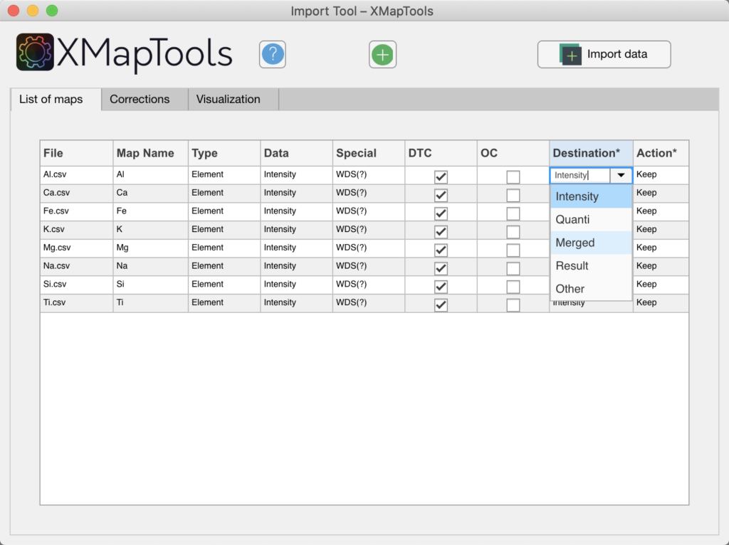
Figure: If maps are expressed in mass of elements, the destination should be changed from 'Intensity' to 'Merged'.

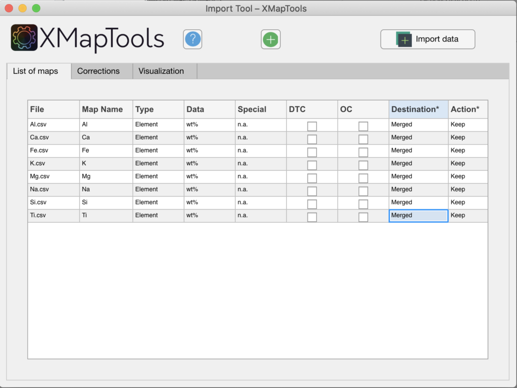
Figure: In this example the destination for each map has been set to 'Merged'.

Step 2: Data conversion (optional)

The compositional maps should ideally be expressed in oxide wt%. if the imported maps are in µg/g or wt% of elements, a conversion step can be required to calculate structural formulas.

In the primary menu, select the dataset Imported_Maps and then right-click on its name. Select the option Convert to open the Converter module.

Select the conversion method in the Converter tool and press the Apply button.

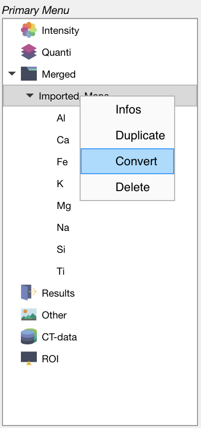
Figure: Select a dataset and then right-click to open the Converter from the primary menu.

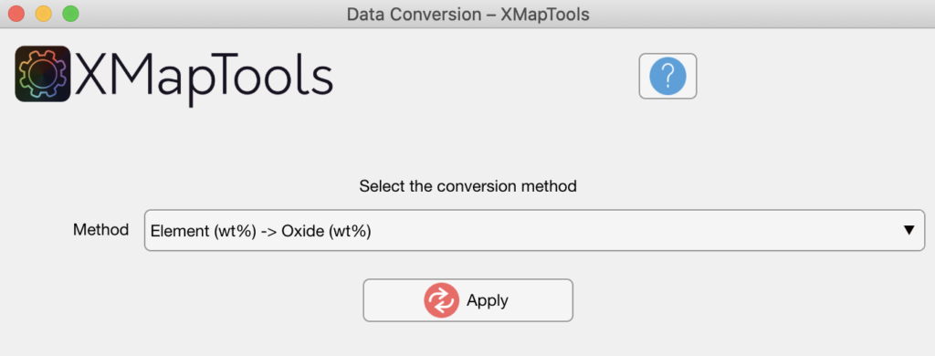
Figure: Data conversion tool. In this example data are converted from element wt% to oxide wt%.

Step 3: Classification of quantitative data

Step 3.1: Create a training set

Display a map from the imported dataset using the Primary Menu and open the Classify tab. Select Training Set (Classification) in the Secondary Menu and press the Add button in Classify and select the phases. Press again the Add button to create a new mask definition in the training set. This operation can be repeated until the correct number of phases is reached. Each mask definition can be deleted by right-clicking on the name and selecting Delete.

You can rename each mask definition by double-clicking on his name in the Secondary Menu. Press Add in Classify when a mask definition is selected to add a region-of-interest (ROI).

Step 3.2: Add maps for classification

Select the dataset in the category Merged of the Primary Menu and press the Add Maps for Classification button to add all the maps of the dataset in the list that will be used by the classification function.

Step 3.3: Classification

Select a dataset in the Merged category of the Primary Menu and a Training Set in the Secondary Menu. Pick an algorithm in the tab Classify and press the Classify button. Note that the Classify button is only available when an appropriate dataset and training set are selected in the primary and secondary menus.

Step 4: Splitting a merged dataset using a maskfile

The imported dataset available in the Merged data category has to be divided into maps for each mask that will be stored under the Quanti data category.

Select a mask file in the Secondary Menu. Select the dataset in Merged and then right-click on its name. Select the Split (using maskfile) option.

The results are stored under the Quanti category as individual dataset, one for each mask. These data sets can be used to calculate maps of structural formulas or other calculations.

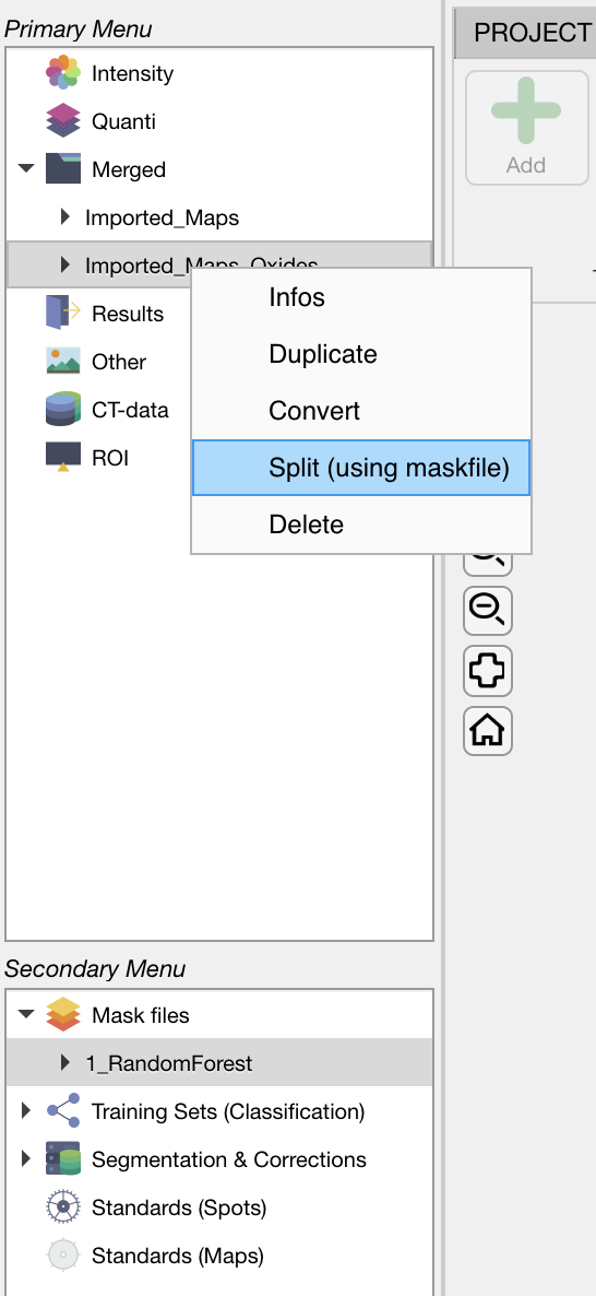
Figure: Select a mask file, then click on the dataset of interest (here Imported_Maps_Oxides) and then right-click on the name for accessing the menu.

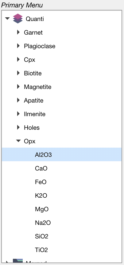
Figure: Results are stored in the category Quanti

Classification

Compositional map classification is the process of categorising and labelling groups of pixels within a dataset based on their composition. It generates a mask image showing the distribution of each mask/class (i.e. features can be mineral/epoxy/glass, etc.).

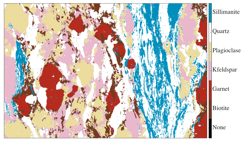
Figure: Example of mask image for a metapelite from the Himalaya published in Lanari & Duesterhoeft (2019). Each feature (mineral) is shown with a colour. Note that all the pixels of this image have been classified.

Classification parameters & algorithms

These tools are used to select an algorithm and maps to be used for classification.

Chemical system: how to add/remove maps?

The goal is to set the map input of the classification function. It is not required to use all available maps for classification; maps containing only noise are usually excluded.

The list of maps used by the classification function is displayed in the text field. The button Add Maps for Classification adds all maps available in the intensity tab of the primary menu. The button Edit Selected Map can have two modes: add (plus icon) or eliminate (minus icon) depending on whether the map selected in the primary menu is already available in the list or not. Clicking "plus" adds the selected map, whereas clicking "minus" eliminates the selected map from the list.

Algorithm selection

The machine learning algorithm used for classification can be selected via the algorithm menu available in the section Classification Parameters.

The following algorithms are available:

• Random Forest: An ensemble learning method for classification constructing a multitude of decision trees during training. The output of the random forest is the class selected by most trees (majority vote).
• Discriminant Analysis: Classification method that assumes that different classes generate data based on different Gaussian distributions. To train a classifier, it estimates the parameters of a Gaussian distribution for each class.
• Naive Bayes: Classification algorithm applying density estimation to the data and generating a probability model. The decision rule is based on the Bayes theorem.
• Support Vector Machine: Data points (p-dimensional vector) are separated into n classes by separating them with a (p-1)-dimensional hyperplane. The algorithm chooses the hyperplane so that the distance from it to the nearest data point on each side is maximised.
• Classification Tree: A decision tree is used as predictive model to classify the input features into classes via a series of decision nodes. Each leaf of the tree is labelled with a class.
• k-Nearest Neighbour: An object is classified by a plurality vote of its neighbours, with the object being assigned to the class most common among its k nearest neighbours.
• k-Means: Classification method that aims to partition n observations into k clusters in which each observation belongs to the cluster with the nearest cluster centroid, serving as a prototype of the cluster.

Principal component analysis (PCA) — Optional

The principal components of a collection of points in a real coordinate space are a sequence of vectors consisting of best-fitting lines, each of them defined as one that minimizes the average squared distance from the points to the line. These directions constitute an orthonormal basis in which different individual dimensions of the data are linearly uncorrelated. The first principal component can equivalently be defined as a direction that maximizes the variance of the projected data. Principal component analysis (PCA) is the process of computing the principal components and using them to perform a change of basis on the data.

The button Generate Maps of the Principal Components (PCA) generates a map for each principal component and stores them in the section Other of the primary menu.

If the tick-box incl. PCA is selected, the maps of principal components are included as additional dimensions for the classification. Example: if 8 intensity maps are considered, a total of 14 maps of PC are added to the classification input, 7 for a normal PCA and 7 for a normalised PCA.

Training and classification

A training set must be selected in the secondary menu in order to activate the classification button.

The button Classify (Train a Classifier & Classify) trains a new classifier and performs the classification using the algorithm selected in the menu and the specified set of maps.

A new figure containing up to four plots will open and be continuously updated during classification. Do not close this figure until the classification is complete, otherwise the plots will not be displayed.

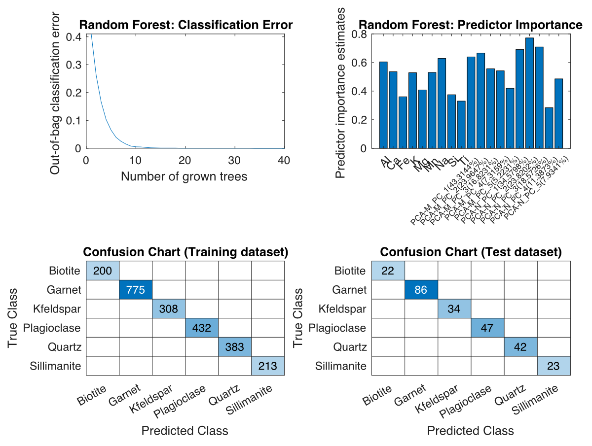
Figure: Plots for classification using the Random Forest algorithm. Top left: out-of-bag classification error vs. number of trees grown. Top right: Predictor importance. Bottom left: Confusion map of the training data set. Bottom right: Confusion plot of the test dataset.

Once the classification is achieved, a new mask file is generated and stored under Mask files in the secondary menu. The mask file is automatically selected and the mask image displayed in the main figure.

Filtering options

The following options apply to a given mask file. Select a mask file in the secondary menu to apply changes.

Select the option to hide pixels having a class probability lower than a given threshold for the selected mask file. Set the probability threshold used for hiding pixels. This value should range between 0 and 1.

The button Create new mask file with pixels filtered by probability generates a new mask file after filtering. This option replaces the BCR correction available in XMapTools 3 and is more adequate as only the misclassified pixels are excluded.

Mask analysis & visualisation

The modes of each class within a given region-of-interest can be exported using the tools provided in this section. Modes are given as surface percentage calculated using the number of pixels of each class. For minerals, this can be eventually extrapolated to volume fraction as discussed in Lanari & Engi (2017).

Select the ROI shape to be used to extract the local modes from the dropdown menu.

The button Add ROI allows a new region-of-interest (ROI) to be drawn on the figure. Note that a mask file must be selected before activating this mode. Results are displayed in the right window as a table containing the modes and number of pixels for each class and as a pie diagram.

The following ROI shapes are available:

• Rectangle: click to select the first corner and drag the mouse to the opposite corner defining a rectangle
• Polygon: click successively on the image to draw a polygon; right-clicking validates and closes automatically the shape

The button Plot Compositions generates a plot using the data selected in the primary menu (either intensity, or a merged map) and the mask file selected in the secondary menu.

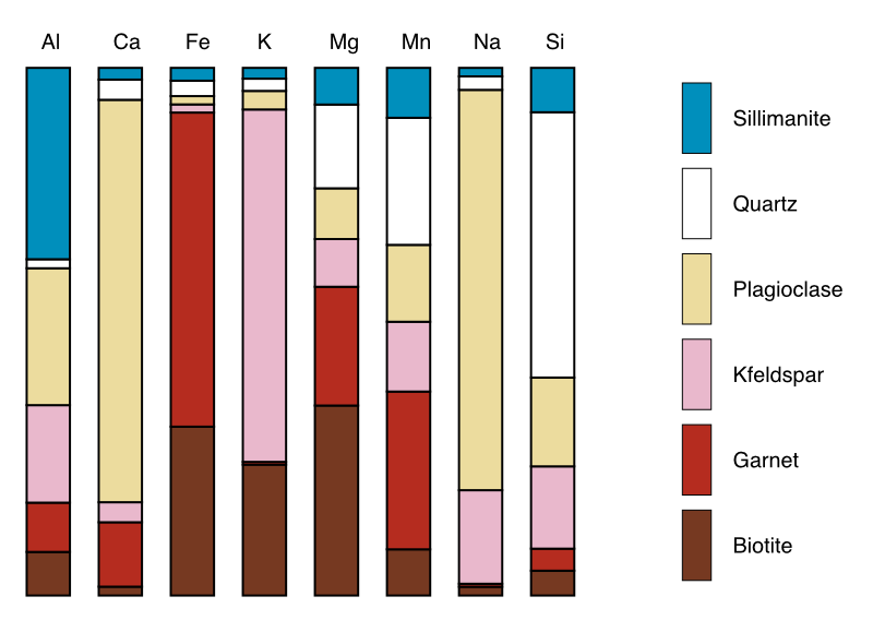
Figure: Example of compositional plot generated using a merged map (expressed in oxide wt%) and a mask file.

Calibration (EPMA)

The following steps are required to convert raw data (e.g. X-ray maps) into maps of chemical composition:

• Import standard data as spot analyses for the calibration of EPMA data
• Check/adjust/add standard data
• Calibrate using the Calibration Assistant for EPMA data

Standard data

The spot analyses used as internal standards in the calibration of EPMA data are referred to as "standards" in the following as they permit to define a calibration curve that correlates X-ray intensities to composition (e.g. expressed in oxide/element wt%).

It is necessary to import the standards from a standard file, check their positions and eventually correct, check the chemical compositions and eventually create new standards. All these steps can be achieved in XMapTools 4.

File Standards.txt

The file Standards.txt contains (i) the map coordinates and (ii) the spot analyses used for the standardisation. The map coordinates must be listed within a single row below the keyword >1. The oxide order is set below the keyword >2. X and Y must be the two last labels and must be listed in this specific order. The internal standards analyses are listed below the keyword >3 corresponding to the oxide order defined above (keyword >2).

>1 Here paste the image coordinates (Xmin Xmax Ymax Ymin)
56.739 57.239 43.691 43.371

>2 Here define the oxides order
SiO2 MgO FeO Al2O3 X Y

>3 Here paste the analyses 
25.4800 11.260 29.050 21.1400 1.4800 68.310 39.999
52.9400 3.5300 3.0200 24.2300 0.0197 68.310 39.535
52.5800 3.6300 2.7900 24.7200 0.0195 68.331 39.511

Import standards

The button Import (Import spots for Standards (from file)) is used to import standards from a file.

The box Import from Standards.txt is selected by default allowing the file 'Standards.txt' to be read automatically. If the file containing the standard data has a different name, unselect the box and it will be possible to select a file in the Pick a file pop-up window. At the moment all standards need to be stored within a single file. It is not possible to import standards from different files as existing standards will be eliminated when a new file is loaded.

Once loaded, standards are displayed on the main map with a label including the spot number and several plots are produced and shown in the category "Standards" of the live display module. You can get this global visualisation at any stage by selecting Standards (Spots) in the Secondary Menu. Three plots are produced if an element is selected in the primary menu, from top to bottom: (1) a plot showing intensity/composition versus sequence of standard to visualise if there is a good match between the standard compositions and the intensity values of the matching pixels; (2 and 3) two correlation maps, one for the selected element in the primary menu and a second one considering all elements.

Adjusting standard positions

To adjust the positions, display the map of a diagnostic element (Intensity) and select Standards (Spots) in the secondary menu. The two correlation maps should show a maximum value in yellow and the blue spot representing the current position should be centred on this optimum.

To adjust the position of the standards (all at once), put the mouse cursor over the blue circle showing up a transparent circle. Click on it and move the blue circle to the new position. The values in the two white fields on top will be adjusted. Then click on the button Refresh (important) to update the standard positions. The Refresh button is only available when standard positions have been changed and need to be saved.

Note: If no good correlation exists for a given element, the higher value of the second figure could not represent the optimal position.

Adding new standard point(s)

It is possible to add new standard points directly in XMapTools. Note that these will not be saved to the file Standards.txt, and if the file is loaded again all changes will be lost.

The button Add standard point adds a new standard at selected coordinates, set by clicking on the map after pressing the button. Compositional data can be filled directly in the table, when this standard is selected.

Procedure:

• Select an element map (e.g. SiO₂ for adding a spot of quartz) and select the item Standards (Spots) in the secondary menu
• Press the button Add Standard Point
• Click on the map at the position to add the new standard point
• (Optional) It is possible to adjust the position of any manual standard by moving the blue spot (transparent circle) or its label (cross-shaped cursor)
• The new standard point is automatically selected in the Secondary Menu and the composition table shown on the right side
• You can enter manually the oxide (wt%) composition of the new standard in the column 'wt%' in blue. The X-ray intensity of the corresponding pixel is already available in the 'Int' column
• There is nothing more to do — all data are automatically saved
• (Optional) You can rename any standard by double clicking on its name in the secondary menu

Map calibration

A calibration step, also known as standardisation, is required to convert intensity maps into compositional maps (Lanari et al. 2019).

All minerals/objects are calibrated at the same time in XMapTools 4. Therefore it is required to select a Mask File in the Secondary Menu to activate the button Calibrate.

The approach implemented in XMapTools 4 provides a module for auto multi-phase calibration. The button Calibrate opens the Calibration Assistant for EPMA Data. This button is only available when a mask file is selected in the Secondary Menu.

For more detailed information on the Calibration Assistant, refer to the embedded documentation accessible from the assistant.

Calibration assistant (EPMA)

The new approach implemented in XMapTools 4 provides a module for automatic multi-phase calibration. The general procedure is described in De Andrade et al. (2006) and an advanced approach including pseudo-background correction is described in Lanari et al. (2019).

Strategy: advantages and pitfalls

An automatic calibration is performed taking into account all spot analyses and all masks when the Calibrate button is pressed. The new algorithm first performs a general fit including all standards and then adjusts the calibration for each mineral. All calibration curves, including those for the general fit, are accessible from the tree menu.

When you press the Apply Standardisation button, all the calibrated maps for each mineral as well as a merged map are created and sent back to XMapTools.

Important

First make sure you check the quality of the calibration curves generated by the auto function!

The automatic function will work if all minerals have been measured with at least a few spot analyses and if there is at least one mineral with a composition above 1 wt% for each element. If a mineral or other feature (e.g. fracture) has no spot analyses, the program extrapolates a calibration from the general fit and thus "predicts" a composition. At this stage this composition is likely to be off because matrix effects are ignored!

INFO

• If you close the Calibration Assistant window, no calibrated data or calibration settings will be saved.
• When you press Apply Standardisation, all maps are sent to XMapTools.

Displaying calibration curves

The Calibration Assistant for EPMA Data opens when the Calibrate button in XMapTools is pressed.

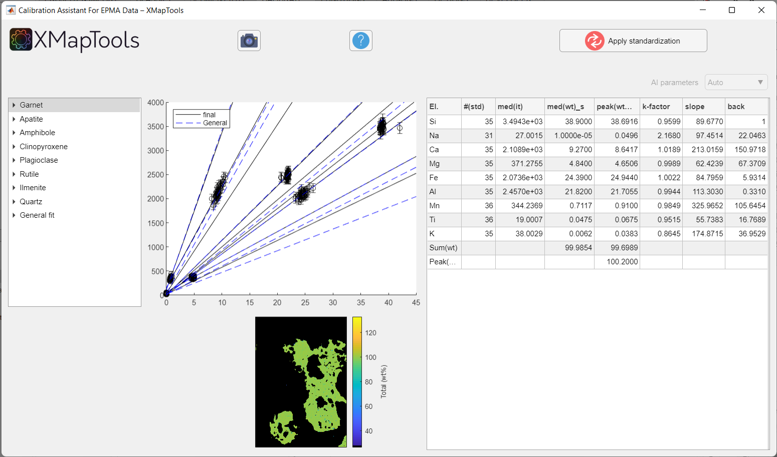
Figure: Example calibration for a clinopyroxene-garnet amphibolite metapelite of the Brasília orogen (Brazil), published in Tedeschi et al. (2017). Note that the calibration curves for all minerals are displayed when the window pops up.

Use the tree menu on the left to navigate through the list of minerals and elements and to view calibration curves.

When you select a mineral from the tree menu, a single plot showing the sum of elements/oxides (total wt%) is displayed. The plot in the middle shows all calibration curves, for all elements of the selected mineral. Some data is displayed in a table:

Column	Description
El.	Element name (of the map); includes sum(wt%) and Peak(SumOx) labels
#(std)	Number of internal standards (spot analyses) used to calibrate the phase
med(it)	Median intensity value for all pixels of the selected mineral for each element
med(wt)_s	Median composition of all internal standard measurements (spot analyses)
mode(wt)_m	Most common composition in the calibrated pixels
k factor	Difference between the general fit calibration and the final mineral calibration (1 = identical)
Slope	Slope of the calibration curve
Background	Intercept of the calibration curve

TIP

The values of mode(SumOx) and Sum(wt) may be different, in which case the median is likely to be influenced by non-Gaussian signals and may not be comparable with the median of the spot analyses. The comparison of both columns can be used to detect potential calibration problems.

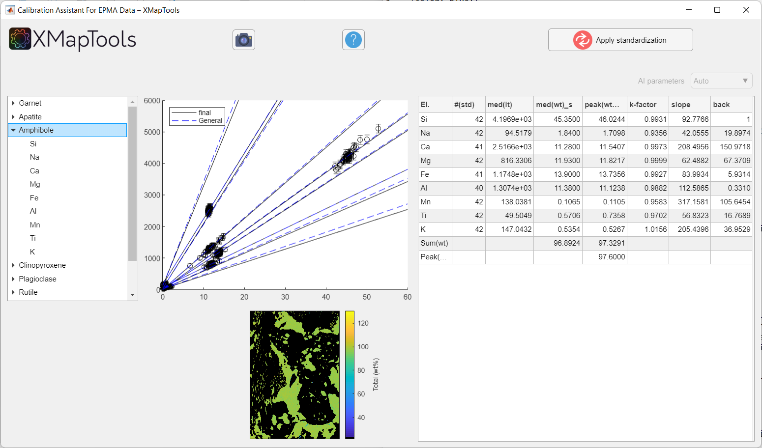
Figure: Example of calibration when a mineral is selected. All calibration curves for a given mineral are displayed.

To view a specific calibration curve (for a particular element), expand the menu by clicking on the small arrow to the left of the mineral name and select an element. The corresponding calibration curve is displayed together with the corresponding quantitative map (oxide wt-%).

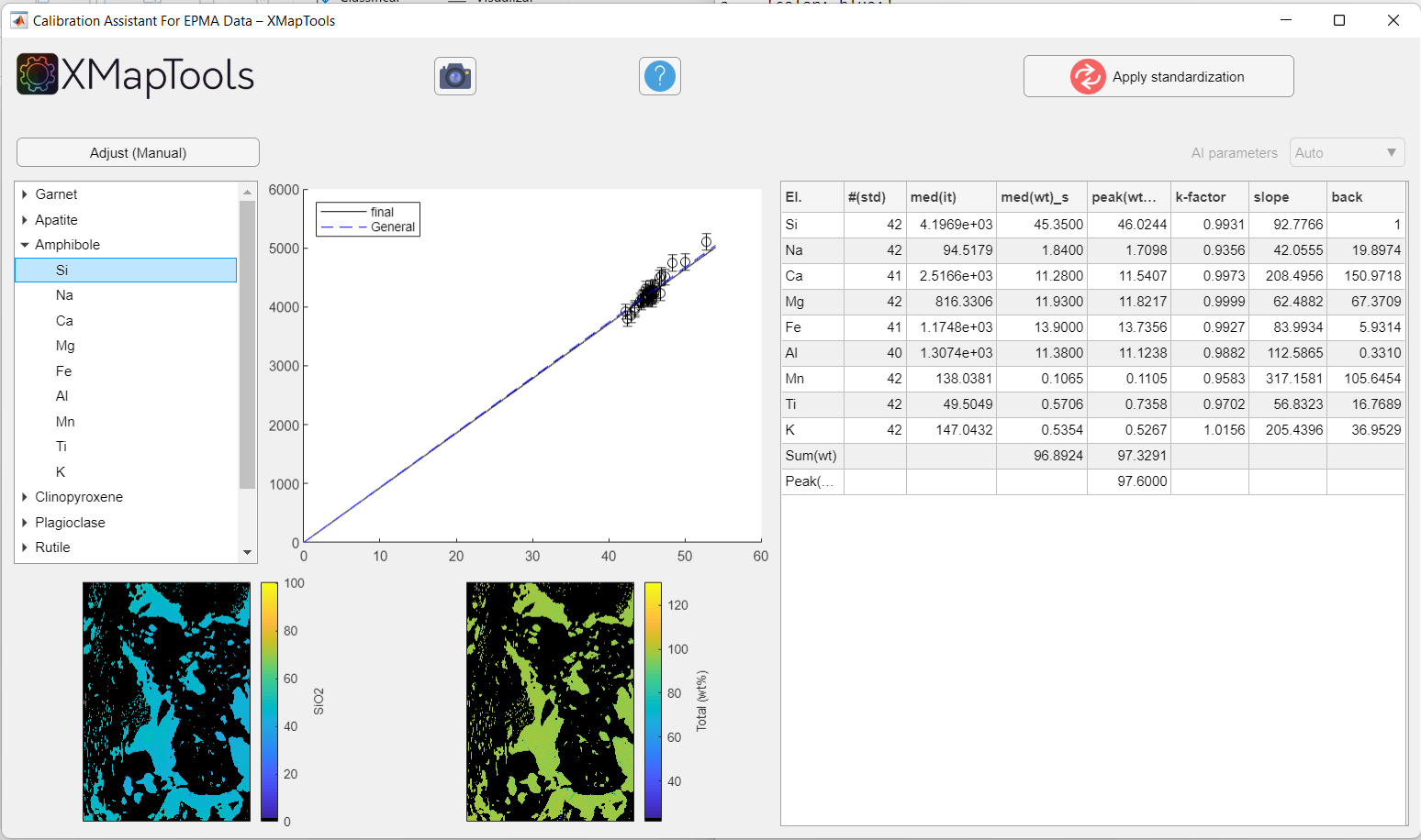
Figure: Example when an element of a given mineral phase is selected. The calibration curve and quantitative map for a given element are displayed.

Adjusting a calibration curve

When an element is selected, the Adjust button appears above the tree menu.

Clicking this button displays two fields containing the values for background and slope:

Values can be changed manually by entering new values in the appropriate field. Press Enter to calculate and display the new calibration curve on the graph (this operation may take a few seconds).

Displaying results of the general fit

Selecting General Fit (last option in the tree menu) will display a plot of the calibration curves for all elements. It is not possible to adjust the calibration curves in the general fit. This fit is automatically performed first by the program and is no longer used once the calibration of each mineral has been achieved.

Apply calibration

After checking each calibration curve and adjusting if necessary, use the Apply Standardisation button to generate the calibrated maps.

By applying the standardisation:

• The Quanti option in the Primary Menu becomes available, where quantitative maps in element/oxide wt-% of each phase can be displayed.
• The Merged option in the Primary Menu also becomes available. A set of merged maps (i.e. quantitative maps in oxide wt-% for all phases considered together) is automatically generated.

Notes

• Red dots indicate outliers that were not included in the calculation of the calibration curves.
• Moving the cursor over the images brings up a Image Menu at the top right. This menu includes options to zoom, save and copy the images.

Local bulk compositions

A local bulk composition (abbreviation: LBC) represents the bulk composition of a spatial domain in a rock determined by integrating pixel compositions. As discussed in Lanari and Engi (2017), it is necessary to apply a density correction prior to exporting any local bulk composition.

To export local bulk compositions the following steps should be employed:

• Generate a density map
• Generate a merged map (if not available yet)
• Select an area of interest to extract the local bulk composition

Generate a density map

A density map is a map containing density data for each pixel of a map. It is calculated for a given mask file. Select a mask file in the secondary menu.

The button Generate Density Map (from a mask file) allows a density map to be generated from the selected mask file. A mask file should be selected to activate the button. Pressing this button opens a window with predefined average density values (provided that the mineral name was recognised and a reference value available in the internal database; when full names of minerals in English are used, the mineral should be recognised).

Note: mineral density values can be obtained from the website webmineral.com.

A density map will be created and stored under the category Other in the Primary Menu with the name 'Density [maskfile_name]'.

Generate a merged map

Merged maps are maps for which all pixels hold a chemical composition. A merged map is automatically created by the standardisation function in XMapTools 4. If you need to create a merged map manually, follow the procedure below.

In the primary menu, unfold Quanti and select a quanti map (mineral). The button Merge (Merge Quanti Data) in the section Calibrate becomes available. In the window that pops up, select the quanti maps to be merged. Select 'Ok' to generate the merged maps that will be stored in the category Merged.

Select ROI and calculate LBC

A local bulk composition can be calculated from a region-of-interest (ROI). The ROI can be a rectangle or a polygon. The density correction is automatically applied.

Select a merged map in the primary menu and display an element. In the dropdown menu, select the wanted ROI shape: Rectangle ROI or Polygon ROI.

The button Add a ROI for LBC extraction allows a region-of-interest (ROI) to be drawn on the figure. If Rectangle ROI is selected, click on a corner, hold and drag to draw a rectangle. If Polygon ROI is selected, click on the image to draw the polygon and close by selecting the first point or right-clicking.

When a ROI is available, the table containing the local bulk composition appears in the live display module. The first column shows the element list, whereas compositions are listed in the column composition (unit: wt%). Below the table, a pie chart shows the repartition of the elements/oxides by weight.

The ROI can be edited and the composition values in the table and the pie chart are automatically updated.

The density map used is shown in a dropdown menu located in the live display module.

The button Copy Data to clipboard may be used to copy the LBC data from the table. The button Save may be used to save the LBC data as a .txt file.

Approximation of uncertainties for LBC

An uncertainty approximation similar to what is described in Lanari and Engi (2017) is available.

Select a merged map and create a Rectangle ROI. Define the number of simulations Sim (default 100) and the shift Px in pixel (default 20). The shape will be randomly displaced and resized using two random variables calculated from the shift value (assuming a Gaussian distribution and the value of Px as 1 sigma expressed in number of pixels). Click on the button Calculate uncertainties using Monte-Carlo.

The areas used to approximate an uncertainty are plotted in a new figure and the result is shown in the table of the live display module. The column composition shows the original local bulk composition (selected ROI). The column 2std shows the 2 standard deviation value (note that the distributions are usually Gaussian as shown by Lanari & Engi (2017)). The last column shows the mean value of all compositions. This value should match the composition of the original ROI. If not, this means that a Gaussian distribution cannot be assumed for this element and the uncertainty is not correct.

References

• De Andrade, V., Vidal, O., Lewin, E., O'Brien, P., Agard, P. (2006). Quantification of electron microprobe compositional maps of rock thin sections: an optimized method and examples. Journal of Metamorphic Geology, 24, 655–668.
• Lanari, P., & Engi, M. (2017). Local bulk composition effects on metamorphic mineral assemblages, Reviews in Mineralogy and Geochemistry, 83, 55–102.
• Lanari, P., Vho, A., Bovay, T., Airaghi, L., Centrella, S. (2019). Quantitative compositional mapping of mineral phases by electron probe micro-analyser. Geological Society of London, Special Publications, 478, 39–63.